Chapter 8 Object documentation

Documentation is one of the most important aspects of a good package. Without it, users won’t know how to use your package. Documentation is also useful for future-you (so you remember what your functions were supposed to do), and for developers extending your package.

There are multiple forms of documentation. In this chapter, you’ll learn about object documentation, as accessed by ? or help(). Object documentation is a type of reference documentation. It works like a dictionary: while a dictionary is helpful if you want to know what a word means, it won’t help you find the right word for a new situation. Similarly, object documentation is helpful if you already know the name of the object, but it doesn’t help you find the object you need to solve a given problem. That’s one of the jobs of vignettes, which you’ll learn about in the next chapter.

R provides a standard way of documenting the objects in a package: you write .Rd files in the man/ directory. These files use a custom syntax, loosely based on LaTeX, and are rendered to HTML, plain text and pdf for viewing. Instead of writing these files by hand, we’re going to use roxygen2 which turns specially formatted comments into .Rd files. The goal of roxygen2 is to make documenting your code as easy as possible. It has a number of advantages over writing .Rd files by hand:

Code and documentation are intermingled so that when you modify your code, you’re reminded to also update your documentation.
Roxygen2 dynamically inspects the objects that it documents, so you can skip some boilerplate that you’d otherwise need to write by hand.
It abstracts over the differences in documenting different types of objects, so you need to learn fewer details.

As well as generating .Rd files, roxygen2 can also manage your NAMESPACE and the Collate field in DESCRIPTION. This chapter discusses .Rd files and the collate field. NAMESPACE describes how you can use roxygen2 to manage your NAMESPACE, and why you should care.

8.1 The documentation workflow

In this section, we’ll first go over a rough outline of the complete documentation workflow. Then, we’ll dive into each step individually. There are four basic steps:

Add roxygen comments to your .R files.
Run devtools::document() (or press Ctrl/Cmd + Shift + D in RStudio) to convert roxygen comments to .Rd files. (devtools::document() calls roxygen2::roxygenise() to do the hard work.)
Preview documentation with ?.
Rinse and repeat until the documentation looks the way you want.

The process starts when you add roxygen comments to your source file: roxygen comments start with #' to distinguish them from regular comments. Here’s documentation for a simple function:

#' Add together two numbers.
#' 
#' @param x A number.
#' @param y A number.
#' @return The sum of \code{x} and \code{y}.
#' @examples
#' add(1, 1)
#' add(10, 1)
add <- function(x, y) {
  x + y
}

Pressing Ctrl/Cmd + Shift + D (or running devtools::document()) will generate a man/add.Rd that looks like:

% Generated by roxygen2 (4.0.0): do not edit by hand
\name{add}
\alias{add}
\title{Add together two numbers}
\usage{
add(x, y)
}
\arguments{
  \item{x}{A number}

  \item{y}{A number}
}
\value{
The sum of \code{x} and \code{y}
}
\description{
Add together two numbers
}
\examples{
add(1, 1)
add(10, 1)
}

If you’re familiar with LaTeX, this should look familiar since the .Rd format is loosely based on it. You can read more about the Rd format in the R extensions manual. Note the comment at the top of the file: it was generated by code and shouldn’t be modified. Indeed, if you use roxygen2, you’ll rarely need to look at these files.

When you use ?add, help("add"), or example("add"), R looks for an .Rd file containing \alias{"add"}. It then parses the file, converts it into HTML and displays it. Here’s what the result looks like in RStudio:

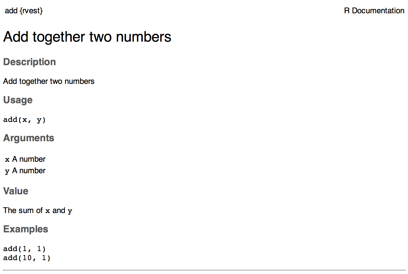
(Note you can preview development documentation because devtools overrides the usual help functions to teach them how to work with source packages. If the documentation doesn’t appear, make sure that you’re using devtools and that you’ve loaded the package with devtools::load_all().)

8.2 Alternative documentation workflow

The first documentation workflow is very fast, but it has one limitation: the preview documentation pages will not show any links between pages. If you’d like to also see links, use this workflow:

Add roxygen comments to your .R files.
Click in the build pane or press Ctrl/Cmd + Shift + B. This completely rebuilds the package, including updating all the documentation, installs it in your regular library, then restarts R and reloads your package. This is slow but thorough.
Preview documentation with ?.
Rinse and repeat until the documentation looks the way you want.

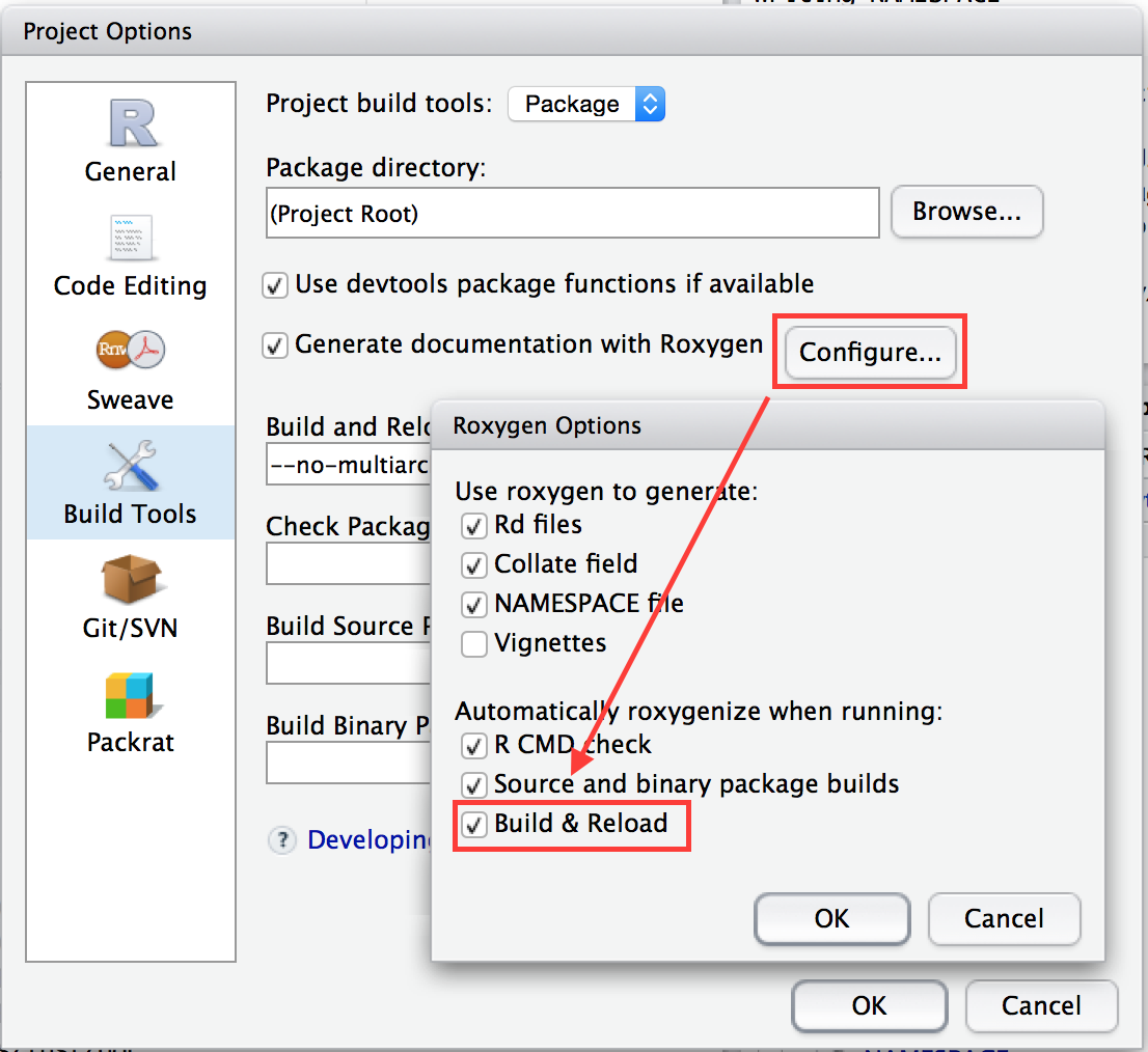
If this workflow doesn’t seem to be working, check your project options in RStudio. Old versions of devtools and RStudio did not automatically update the documentation when the package was rebuilt:

8.3 Roxygen comments

Roxygen comments start with #' and come before a function. All the roxygen lines preceding a function are called a block. Each line should be wrapped in the same way as your code, normally at 80 characters.

Blocks are broken up into tags, which look like @tagName details. The content of a tag extends from the end of the tag name to the start of the next tag (or the end of the block). Because @ has a special meaning in roxygen, you need to write @@ if you want to add a literal @ to the documentation (this is mostly important for email addresses and for accessing slots of S4 objects).

Each block includes some text before the first tag.⁷ This is called the introduction, and is parsed specially:

The first sentence becomes the title of the documentation. That’s what you see when you look at help(package = mypackage) and is shown at the top of each help file. It should fit on one line, be written in sentence case, but not end in a full stop.
The second paragraph is the description: this comes first in the documentation and should briefly describe what the function does.
The third and subsequent paragraphs go into the details: this is a (often long) section that is shown after the argument description and should go into detail about how the function works.

All objects must have a title and description. Details are optional.

Here’s an example showing what the introduction for sum() might look like if it had been written with roxygen:

#' Sum of vector elements.
#' 
#' \code{sum} returns the sum of all the values present in its arguments.
#' 
#' This is a generic function: methods can be defined for it directly or via the
#' \code{\link{Summary}} group generic. For this to work properly, the arguments
#' \code{...} should be unnamed, and dispatch is on the first argument.
sum <- function(..., na.rm = TRUE) {}

\code{} and \link{} are formatting commands that you’ll learn about in formatting. I’ve been careful to wrap the roxygen block so that it’s less than 80 characters wide. You can do that automatically in Rstudio with Ctrl/Cmd + Shift + / (or from the menu, code | re-flow comment).

You can add arbitrary sections to the documentation with the @section tag. This is a useful way of breaking a long details section into multiple chunks with useful headings. Section titles should be in sentence case, must be followed by a colon, and they can only be one line long.

#' @section Warning:
#' Do not operate heavy machinery within 8 hours of using this function.

There are two tags that make it easier for people to navigate between help files:

@seealso allows you to point to other useful resources, either on the web, \url{http://www.r-project.org}, in your package \code{\link{functioname}}, or another package \code{\link[packagename]{functioname}}.
If you have a family of related functions where every function should link to every other function in the family, use @family. The value of @family should be plural.

For sum, these components might look like:

#' @family aggregate functions
#' @seealso \code{\link{prod}} for products, \code{\link{cumsum}} for cumulative
#'   sums, and \code{\link{colSums}}/\code{\link{rowSums}} marginal sums over
#'   high-dimensional arrays.

Two other tags make it easier for the user to find documentation:

@aliases alias1 alias2 ... adds additional aliases to the topic. An alias is another name for the topic that can be used with ?.
@keywords keyword1 keyword2 ... adds standardised keywords. Keywords are optional, but if present, must be taken from a predefined list found in file.path(R.home("doc"), "KEYWORDS").

Generally, keywords are not that useful except for @keywords internal. Using the internal keyword removes the function from the package index and disables some of its automated tests. It’s common to use @keywords internal for functions that are of interest to other developers extending your package, but not most users.

Other tags are situational: they vary based on the type of object that you’re documenting. The following sections describe the most commonly used tags for functions, packages and the various methods, generics and objects used by R’s three OO systems.

8.4 Documenting functions

Functions are the most commonly documented object. As well as the introduction block, most functions have three tags: @param, @examples and @return.

@param name description describes the function’s inputs or parameters. The description should provide a succinct summary of the type of the parameter (e.g., string, numeric vector) and, if not obvious from the name, what the parameter does.

The description should start with a capital letter and end with a full stop. It can span multiple lines (or even paragraphs) if necessary. All parameters must be documented.

You can document multiple arguments in one place by separating the names with commas (no spaces). For example, to document both x and y, you can write @param x,y Numeric vectors..
@examples provides executable R code showing how to use the function in practice. This is a very important part of the documentation because many people look at the examples first. Example code must work without errors as it is run automatically as part of R CMD check.

For the purpose of illustration, it’s often useful to include code that causes an error. \dontrun{} allows you to include code in the example that is not run. (You used to be able to use \donttest{} for a similar purpose, but it’s no longer recommended because it actually is tested.)

Instead of including examples directly in the documentation, you can put them in separate files and use @example path/relative/to/package/root to insert them into the documentation. (Note that the @example tag here has no ‘s’.)
@return description describes the output from the function. This is not always necessary, but is a good idea if your function returns different types of output depending on the input, or if you’re returning an S3, S4 or RC object.

We could use these new tags to improve our documentation of sum() as follows:

#' Sum of vector elements.
#'
#' \code{sum} returns the sum of all the values present in its arguments.
#'
#' This is a generic function: methods can be defined for it directly
#' or via the \code{\link{Summary}} group generic. For this to work properly,
#' the arguments \code{...} should be unnamed, and dispatch is on the
#' first argument.
#'
#' @param ... Numeric, complex, or logical vectors.
#' @param na.rm A logical scalar. Should missing values (including NaN)
#'   be removed?
#' @return If all inputs are integer and logical, then the output
#'   will be an integer. If integer overflow
#'   \url{http://en.wikipedia.org/wiki/Integer_overflow} occurs, the output
#'   will be NA with a warning. Otherwise it will be a length-one numeric or
#'   complex vector.
#'
#'   Zero-length vectors have sum 0 by definition. See
#'   \url{http://en.wikipedia.org/wiki/Empty_sum} for more details.
#' @examples
#' sum(1:10)
#' sum(1:5, 6:10)
#' sum(F, F, F, T, T)
#'
#' sum(.Machine$integer.max, 1L)
#' sum(.Machine$integer.max, 1)
#'
#' \dontrun{
#' sum("a")
#' }
sum <- function(..., na.rm = TRUE) {}

Indent the second and subsequent lines of a tag so that when scanning the documentation it’s easy to see where one tag ends and the next begins. Tags that always span multiple lines (like @example) should start on a new line and don’t need to be indented.

8.5 Documenting datasets

See documenting data.

8.6 Documenting packages

You can use roxygen to provide a help page for your package as a whole. This is accessed with package?foo, and can be used to describe the most important components of your package. It’s a useful supplement to vignettes, as described in the next chapter.

There’s no object that corresponds to a package, so you need to document NULL, and then manually label it with @docType package and @name <package-name>. This is also an excellent place to use the @section tag to divide up page into useful categories.

#' foo: A package for computating the notorious bar statistic.
#'
#' The foo package provides three categories of important functions:
#' foo, bar and baz.
#' 
#' @section Foo functions:
#' The foo functions ...
#'
#' @docType package
#' @name foo
NULL
#> NULL

I usually put this documentation in a file called <package-name>.R. It’s also a good place to put the package level import statements that you’ll learn about in imports.

8.7 Documenting classes, generics and methods

It’s relatively straightforward to document classes, generics and methods. The details vary based on the object system you’re using. The following sections give the details for the S3, S4 and RC object systems.

8.7.1 S3

S3 generics are regular functions, so document them as such. S3 classes have no formal definition, so document the constructor function. It is your choice whether or not to document S3 methods. You don’t need to document methods for simple generics like print(). But if your method is more complicated or includes additional arguments, you should document it so people know how it works. In base R, you can see examples of documentation for more complex methods like predict.lm(), predict.glm(), and anova.glm().

Older versions of roxygen required explicit @method generic class tags for all S3 methods. From version 3.0.0 onward, this is no longer needed as roxygen2 will figure it out automatically. If you are upgrading, make sure to remove these old tags. Automatic method detection will only fail if the generic and class are ambiguous. For example, is all.equal.data.frame() the equal.data.frame method for all, or the data.frame method for all.equal? If this happens, you can disambiguate with e.g. @method all.equal data.frame.

8.7.2 S4

Document S4 classes by adding a roxygen block before setClass(). Use @slot to document the slots of the class in the same way you use @param to describe the parameters of a function. Here’s a simple example:

#' An S4 class to represent a bank account.
#'
#' @slot balance A length-one numeric vector
Account <- setClass("Account",
  slots = list(balance = "numeric")
)

S4 generics are also functions, so document them as such. S4 methods are a little more complicated, however. Unlike S3, all S4 methods must be documented. You document them like a regular function, but you probably don’t want each method to have its own documentation page. Instead, put the method documentation in one of three places:

In the class. Most appropriate if the corresponding generic uses single dispatch and you created the class.
In the generic. Most appropriate if the generic uses multiple dispatch and you have written both the generic and the method.
In its own file. Most appropriate if the method is complex, or if you’ve written the method but not the class or generic.

Use either @rdname or @describeIn to control where method documentation goes. See documenting multiple objects in one file for details.

Another consideration is that S4 code often needs to run in a certain order. For example, to define the method setMethod("foo", c("bar", "baz"), ...) you must already have created the foo generic and the two classes. By default, R code is loaded in alphabetical order, but that won’t always work for your situation. Rather than relying on alphabetic ordering, roxygen2 provides an explicit way of saying that one file must be loaded before another: @include. The @include tag gives a space separated list of file names that should be loaded before the current file:

#' @include class-a.R
setClass("B", contains = "A")

Often, it’s easiest to put this at the top of the file. To make it clear that this tag applies to the whole file, and not a specific object, document NULL.

#' @include foo.R bar.R baz.R
NULL

setMethod("foo", c("bar", "baz"), ...)

Roxygen uses the @include tags to compute a topological sort which ensures that dependencies are loaded before they’re needed. It then sets the Collate field in DESCRIPTION, which overrides the default alphabetic ordering. A simpler alternative to @include is to define all classes and methods in aaa-classes.R and aaa-generics.R, and rely on these coming first since they’re in alphabetical order. The main disadvantage is that you can’t organise components into files as naturally as you might want.

Older versions of roxygen2 required explicit @usage, @alias and @docType tags for document S4 objects. However, as of version 3.0.0, roxygen2 generates the correct values automatically so you no longer need to use them. If you’re upgrading from an old version, you can delete these tags.

8.7.3 RC

Reference classes are different to S3 and S4 because methods are associated with classes, not generics. RC also has a special convention for documenting methods: the docstring. The docstring is a string placed inside the definition of the method which briefly describes what it does. This makes documenting RC simpler than S4 because you only need one roxygen block per class.

#' A Reference Class to represent a bank account.
#'
#' @field balance A length-one numeric vector.
Account <- setRefClass("Account",
  fields = list(balance = "numeric"),
  methods = list(
    withdraw = function(x) {
      "Withdraw money from account. Allows overdrafts"
      balance <<- balance - x
    }
  )
)

Methods with doc strings will be included in the “Methods” section of the class documentation. Each documented method will be listed with an automatically generated usage statement and its doc string. Also note the use of @field instead of @slot.

8.8 Special characters

There are three special characters that need special handling if you want them to appear in the final documentation:

@, which usually marks the start of a roxygen tag. Use @@ to insert a literal @ in the final documentation.
%, which usually marks the start of a latex comment which continues to the end of the line. Use \% to insert a literal % in the output document. The escape is not needed in examples.
\, which usually marks the start of a latex escaping. Use \\ to insert a literal \ in the documentation.

8.9 Do repeat yourself

There is a tension between the DRY (don’t repeat yourself) principle of programming and the need for documentation to be self-contained. It’s frustrating to have to navigate through multiple help files in order to pull together all the pieces you need. Roxygen2 provides two ways to avoid repetition in the source, while still assembling everything into one documentation file:

The ability to reuse parameter documentation with @inheritParams.
The ability to document multiple functions in the same place with @describeIn or @rdname

8.9.1 Inheriting parameters from other functions

You can inherit parameter descriptions from other functions using @inheritParams source_function. This tag will bring in all documentation for parameters that are undocumented in the current function, but documented in the source function. The source can be a function in the current package, via @inheritParams function, or another package, via @inheritParams package::function. For example the following documentation:

#' @param a This is the first argument
foo <- function(a) a + 10

#' @param b This is the second argument
#' @inheritParams foo
bar <- function(a, b) {
  foo(a) * 10
}

is equivalent to

#' @param a This is the first argument
#' @param b This is the second argument
bar <- function(a, b) {
  foo(a) * 10
}

Note that inheritance works recursively, so you can inherit documentation from a function that has inherited it from elsewhere.

8.9.2 Documenting multiple functions in the same file

You can document multiple functions in the same file by using either @rdname or @describeIn. However, it’s a technique best used with caution: documenting too many functions in one place leads to confusing documentation. You should use it when functions have very similar arguments, or have complementary effects (e.g., open() and close() methods).

@describeIn is designed for the most common cases:

Documenting methods in a generic.
Documenting methods in a class.
Documenting functions with the same (or similar) arguments.

It generates a new section, named either “Methods (by class)”, “Methods (by generic)” or “Functions”. The section contains a bulleted list describing each function. They’re labelled so that you know what function or method it’s talking about. Here’s an example, documenting an imaginary new generic:

#' Foo bar generic
#'
#' @param x Object to foo.
foobar <- function(x) UseMethod("foobar")

#' @describeIn foobar Difference between the mean and the median
foobar.numeric <- function(x) abs(mean(x) - median(x))

#' @describeIn foobar First and last values pasted together in a string.
foobar.character <- function(x) paste0(x[1], "-", x[length(x)])

An alternative to @describeIn is @rdname. It overrides the default file name generated by roxygen and merges documentation for multiple objects into one file. This gives you the complete freedom to combine documentation as you see fit.

There are two ways to use @rdname. You can add documentation to an existing function:

#' Basic arithmetic
#'
#' @param x,y numeric vectors.
add <- function(x, y) x + y

#' @rdname add
times <- function(x, y) x * y

Or, you can create a dummy documentation file by documenting NULL and setting an informative @name.

#' Basic arithmetic
#'
#' @param x,y numeric vectors.
#' @name arith
NULL
#> NULL

#' @rdname arith
add <- function(x, y) x + y

#' @rdname arith
times <- function(x, y) x * y

8.10 Text formatting reference sheet

Within roxygen tags, you use .Rd syntax to format text. This vignette shows you examples of the most important commands. The full details are described in R extensions.

Note that \ and % are special characters in the Rd format. To insert a literal % or \, escape them with a backslash \\, \%.

8.10.1 Character formatting

\emph{italics}: italics.
\strong{bold}: bold.
\code{r_function_call(with = "arguments")}: r_function_call(with = "arguments") (format inline code)
\preformatted{}: format text as-is, can be used for multi-line code

8.10.2 Links

To other documentation:

\code{\link{function}}: function in this package.
\code{\link[MASS]{abbey}}: function in another package.
\link[=dest]{name}: link to dest, but show name.
\code{\link[MASS:abbey]{name}}: link to function in another package, but show name.
\linkS4class{abc}: link to an S4 class.

To the web:

\url{http://rstudio.com}: a url.
\href{http://rstudio.com}{Rstudio}:, a url with custom link text.
\email{hadley@@rstudio.com} (note the doubled @): an email address.

8.10.3 Lists

Ordered (numbered) lists:

#' \enumerate{
#'   \item First item
#'   \item Second item
#' }

Unordered (bulleted) lists:

#' \itemize{
#'   \item First item
#'   \item Second item
#' }

Definition (named) lists:

#' \describe{
#'   \item{One}{First item}
#'   \item{Two}{Second item}
#' }

8.10.4 Mathematics

You can use standard LaTeX math (with no extensions). Choose between either inline or block display:

\eqn{a + b}: inline equation.
\deqn{a + b}: display (block) equation.

8.10.5 Tables

Tables are created with \tabular{}. It has two arguments:

Column alignment, specified by letter for each column (l = left, r = right, c = centre.)
Table contents, with columns separated by \tab and rows by \cr.

The following function turns an R data frame into the correct format. It ignores column and row names, but should get you started.

tabular <- function(df, ...) {
  stopifnot(is.data.frame(df))

  align <- function(x) if (is.numeric(x)) "r" else "l"
  col_align <- vapply(df, align, character(1))

  cols <- lapply(df, format, ...)
  contents <- do.call("paste",
    c(cols, list(sep = " \\tab ", collapse = "\\cr\n  ")))

  paste("\\tabular{", paste(col_align, collapse = ""), "}{\n  ",
    contents, "\n}\n", sep = "")
}

cat(tabular(mtcars[1:5, 1:5]))
#> \tabular{rrrrr}{
#>   21.0 \tab 6 \tab 160 \tab 110 \tab 3.90\cr
#>   21.0 \tab 6 \tab 160 \tab 110 \tab 3.90\cr
#>   22.8 \tab 4 \tab 108 \tab  93 \tab 3.85\cr
#>   21.4 \tab 6 \tab 258 \tab 110 \tab 3.08\cr
#>   18.7 \tab 8 \tab 360 \tab 175 \tab 3.15
#> }

8.10.6 Notes

Note that it is possible to define the “introduction” sections - the title and description - explicitly, rather than implicitly, using @title and @description tags. I follow the convention of avoiding this, as do many other package authors, so I don’t recommend it - but you should be aware that these tags do exist and may appear in other package-writers’ source code.↩︎