7.2 Environment basics

Generally, an environment is similar to a named list, with four important exceptions:

Every name must be unique.
The names in an environment are not ordered.
An environment has a parent.
Environments are not copied when modified.

Let’s explore these ideas with code and pictures.

7.2.1 Basics

To create an environment, use rlang::env(). It works like list(), taking a set of name-value pairs:

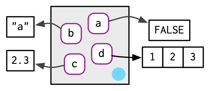
e1 <- env(
  a = FALSE,
  b = "a",
  c = 2.3,
  d = 1:3,
)

Use new.env() to create a new environment. Ignore the hash and size parameters; they are not needed. You cannot simultaneously create and define values; use $<-, as shown below.

The job of an environment is to associate, or bind, a set of names to a set of values. You can think of an environment as a bag of names, with no implied order (i.e. it doesn’t make sense to ask which is the first element in an environment). For that reason, we’ll draw the environment as so:

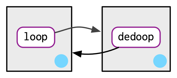
As discussed in Section 2.5.2, environments have reference semantics: unlike most R objects, when you modify them, you modify them in place, and don’t create a copy. One important implication is that environments can contain themselves.

e1$d <- e1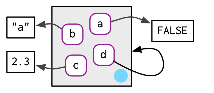

Printing an environment just displays its memory address, which is not terribly useful:

e1
#> <environment: 0x5556a5e81508>

Instead, we’ll use env_print() which gives us a little more information:

env_print(e1)
#> <environment: 0x5556a5e81508>
#> parent: <environment: global>
#> bindings:
#>  * a: <lgl>
#>  * b: <chr>
#>  * c: <dbl>
#>  * d: <env>

You can use env_names() to get a character vector giving the current bindings

env_names(e1)
#> [1] "a" "b" "c" "d"

In R 3.2.0 and greater, use names() to list the bindings in an environment. If your code needs to work with R 3.1.0 or earlier, use ls(), but note that you’ll need to set all.names = TRUE to show all bindings.

7.2.2 Important environments

We’ll talk in detail about special environments in 7.4, but for now we need to mention two. The current environment, or current_env() is the environment in which code is currently executing. When you’re experimenting interactively, that’s usually the global environment, or global_env(). The global environment is sometimes called your “workspace”, as it’s where all interactive (i.e. outside of a function) computation takes place.

To compare environments, you need to use identical() and not ==. This is because == is a vectorised operator, and environments are not vectors.

identical(global_env(), current_env())
#> [1] TRUE

global_env() == current_env()
#> Error in global_env() == current_env(): comparison (1) is possible only for
#> atomic and list types

Access the global environment with globalenv() and the current environment with environment(). The global environment is printed as Rf_GlobalEnv and .GlobalEnv.

7.2.3 Parents

Every environment has a parent, another environment. In diagrams, the parent is shown as a small pale blue circle and arrow that points to another environment. The parent is what’s used to implement lexical scoping: if a name is not found in an environment, then R will look in its parent (and so on). You can set the parent environment by supplying an unnamed argument to env(). If you don’t supply it, it defaults to the current environment. In the code below, e2a is the parent of e2b.

e2a <- env(d = 4, e = 5)
e2b <- env(e2a, a = 1, b = 2, c = 3)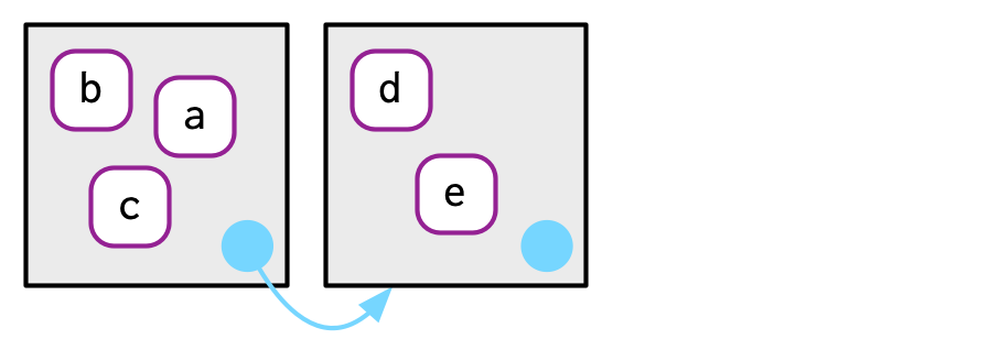

To save space, I typically won’t draw all the ancestors; just remember whenever you see a pale blue circle, there’s a parent environment somewhere.

You can find the parent of an environment with env_parent():

env_parent(e2b)
#> <environment: 0x5556a6ec93f0>
env_parent(e2a)
#> <environment: R_GlobalEnv>

Only one environment doesn’t have a parent: the empty environment. I draw the empty environment with a hollow parent environment, and where space allows I’ll label it with R_EmptyEnv, the name R uses.

e2c <- env(empty_env(), d = 4, e = 5)
e2d <- env(e2c, a = 1, b = 2, c = 3)

The ancestors of every environment eventually terminate with the empty environment. You can see all ancestors with env_parents():

env_parents(e2b)
#> [[1]]   <env: 0x5556a6ec93f0>
#> [[2]] $ <env: global>
env_parents(e2d)
#> [[1]]   <env: 0x5556a84786e0>
#> [[2]] $ <env: empty>

By default, env_parents() stops when it gets to the global environment. This is useful because the ancestors of the global environment include every attached package, which you can see if you override the default behaviour as below. We’ll come back to these environments in Section 7.4.1.

env_parents(e2b, last = empty_env())
#>  [[1]]   <env: 0x5556a6ec93f0>
#>  [[2]] $ <env: global>
#>  [[3]] $ <env: package:rlang>
#>  [[4]] $ <env: package:stats>
#>  [[5]] $ <env: package:graphics>
#>  [[6]] $ <env: package:grDevices>
#>  [[7]] $ <env: package:utils>
#>  [[8]] $ <env: package:datasets>
#>  [[9]] $ <env: package:methods>
#> [[10]] $ <env: Autoloads>
#> [[11]] $ <env: package:base>
#> [[12]] $ <env: empty>

Use parent.env() to find the parent of an environment. No base function returns all ancestors.

7.2.4 Super assignment, `<<-`

The ancestors of an environment have an important relationship to <<-. Regular assignment, <-, always creates a variable in the current environment. Super assignment, <<-, never creates a variable in the current environment, but instead modifies an existing variable found in a parent environment.

x <- 0
f <- function() {
  x <<- 1
}
f()
x
#> [1] 1

If <<- doesn’t find an existing variable, it will create one in the global environment. This is usually undesirable, because global variables introduce non-obvious dependencies between functions. <<- is most often used in conjunction with a function factory, as described in Section 10.2.4.

7.2.5 Getting and setting

You can get and set elements of an environment with $ and [[ in the same way as a list:

e3 <- env(x = 1, y = 2)
e3$x
#> [1] 1
e3$z <- 3
e3[["z"]]
#> [1] 3

But you can’t use [[ with numeric indices, and you can’t use [:

e3[[1]]
#> Error in e3[[1]]: wrong arguments for subsetting an environment

e3[c("x", "y")]
#> Error in e3[c("x", "y")]: object of type 'environment' is not subsettable

$ and [[ will return NULL if the binding doesn’t exist. Use env_get() if you want an error:

e3$xyz
#> NULL

env_get(e3, "xyz")
#> Error in env_get(e3, "xyz"): argument "default" is missing, with no default

If you want to use a default value if the binding doesn’t exist, you can use the default argument.

env_get(e3, "xyz", default = NA)
#> [1] NA

There are two other ways to add bindings to an environment:

env_poke()³⁰ takes a name (as string) and a value:
```
env_poke(e3, "a", 100)
e3$a
#> [1] 100
```

env_bind() allows you to bind multiple values:

env_bind(e3, a = 10, b = 20)
env_names(e3)
#> [1] "x" "y" "z" "a" "b"

You can determine if an environment has a binding with env_has():

env_has(e3, "a")
#>    a 
#> TRUE

Unlike lists, setting an element to NULL does not remove it, because sometimes you want a name that refers to NULL. Instead, use env_unbind():

e3$a <- NULL
env_has(e3, "a")
#>    a 
#> TRUE

env_unbind(e3, "a")
env_has(e3, "a")
#>     a 
#> FALSE

Unbinding a name doesn’t delete the object. That’s the job of the garbage collector, which automatically removes objects with no names binding to them. This process is described in more detail in Section 2.6.

See get(), assign(), exists(), and rm(). These are designed interactively for use with the current environment, so working with other environments is a little clunky. Also beware the inherits argument: it defaults to TRUE meaning that the base equivalents will inspect the supplied environment and all its ancestors.

7.2.6 Advanced bindings

There are two more exotic variants of env_bind():

env_bind_lazy() creates delayed bindings, which are evaluated the first time they are accessed. Behind the scenes, delayed bindings create promises, so behave in the same way as function arguments.
```
env_bind_lazy(current_env(), b = {Sys.sleep(1); 1})

system.time(print(b))
#> [1] 1
#>    user  system elapsed 
#>   0.001   0.000   1.001
system.time(print(b))
#> [1] 1
#>    user  system elapsed 
#>       0       0       0
```
The primary use of delayed bindings is in autoload(), which allows R packages to provide datasets that behave like they are loaded in memory, even though they’re only loaded from disk when needed.
env_bind_active() creates active bindings which are re-computed every time they’re accessed:
```
env_bind_active(current_env(), z1 = function(val) runif(1))

z1
#> [1] 0.0808
z1
#> [1] 0.834
```
Active bindings are used to implement R6’s active fields, which you’ll learn about in Section 14.3.2.

See ?delayedAssign() and ?makeActiveBinding().

7.2.7 Exercises

List three ways in which an environment differs from a list.
Create an environment as illustrated by this picture.
Create a pair of environments as illustrated by this picture.
Explain why e[[1]] and e[c("a", "b")] don’t make sense when e is an environment.
Create a version of env_poke() that will only bind new names, never re-bind old names. Some programming languages only do this, and are known as single assignment languages.

What does this function do? How does it differ from <<- and why might you prefer it?

rebind <- function(name, value, env = caller_env()) {
  if (identical(env, empty_env())) {
    stop("Can't find `", name, "`", call. = FALSE)
  } else if (env_has(env, name)) {
    env_poke(env, name, value)
  } else {
    rebind(name, value, env_parent(env))
  }
}
rebind("a", 10)
#> Error: Can't find `a`
a <- 5
rebind("a", 10)
a
#> [1] 10

You might wonder why rlang has env_poke() instead of env_set(). This is for consistency: _set() functions return a modified copy; _poke() functions modify in place.↩︎