23.3 Microbenchmarking
A microbenchmark is a measurement of the performance of a very small piece of code, something that might take milliseconds (ms), microseconds (µs), or nanoseconds (ns) to run. Microbenchmarks are useful for comparing small snippets of code for specific tasks. Be very wary of generalising the results of microbenchmarks to real code: the observed differences in microbenchmarks will typically be dominated by higher-order effects in real code; a deep understanding of subatomic physics is not very helpful when baking.
A great tool for microbenchmarking in R is the bench package (Hester 2018). The bench package uses a a high precision timer, making it possible to compare operations that only take a tiny amount of time. For example, the following code compares the speed of two approaches to computing a square root.
x <- runif(100)
(lb <- bench::mark(
  sqrt(x),
  x ^ 0.5
))
#> # A tibble: 2 x 6
#>   expression      min   median `itr/sec` mem_alloc `gc/sec`
#>   <bch:expr> <bch:tm> <bch:tm>     <dbl> <bch:byt>    <dbl>
#> 1 sqrt(x)    403.96ns 510.42ns  1789570.      848B        0
#> 2 x^0.5        2.29µs   2.42µs   404899.      848B        0
By default, bench::mark() runs each expression at least once (min_iterations = 1), and at most enough times to take 0.5 s (min_time = 0.5). It checks that each run returns the same value which is typically what you want microbenchmarking; if you want to compare the speed of expressions that return different values, set check = FALSE.
23.3.1 bench::mark() results
bench::mark() returns the results as a tibble, with one row for each input expression, and the following columns:
min,mean,median,max, anditr/secsummarise the time taken by the expression. Focus on the minimum (the best possible running time) and the median (the typical time). In this example, you can see that using the special purposesqrt()function is faster than the general exponentiation operator.You can visualise the distribution of the individual timings with
plot():plot(lb) #> Loading required namespace: tidyr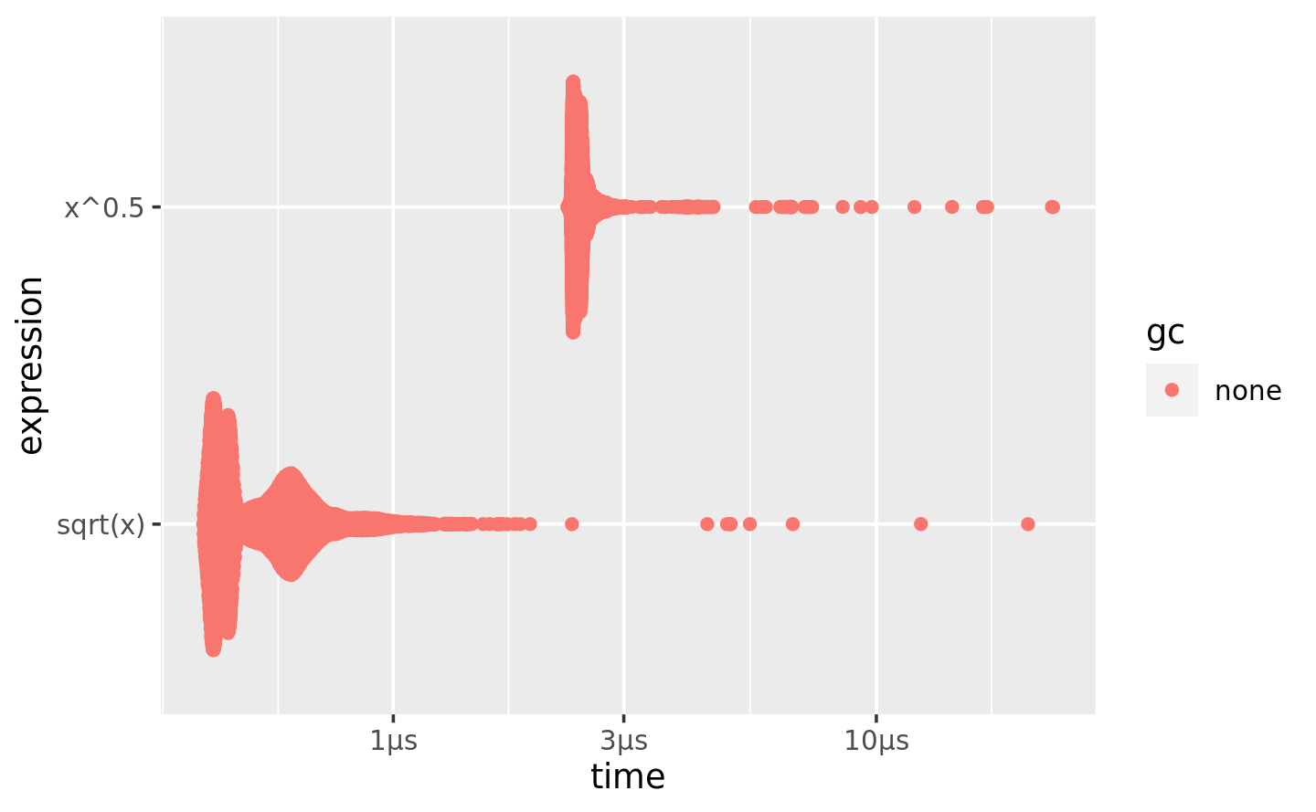
The distribution tends to be heavily right-skewed (note that the x-axis is already on a log scale!), which is why you should avoid comparing means. You’ll also often see multimodality because your computer is running something else in the background.
mem_alloctells you the amount of memory allocated by the first run, andn_gc()tells you the total number of garbage collections over all runs. These are useful for assessing the memory usage of the expression.n_itrandtotal_timetells you how many times the expression was evaluated and how long that took in total.n_itrwill always be greater than themin_iterationparameter, andtotal_timewill always be greater than themin_timeparameter.result,memory,time, andgcare list-columns that store the raw underlying data.
Because the result is a special type of tibble, you can use [ to select just the most important columns. I’ll do that frequently in the next chapter.
lb[c("expression", "min", "median", "itr/sec", "n_gc")]
#> # A tibble: 2 x 4
#>   expression      min   median `itr/sec`
#>   <bch:expr> <bch:tm> <bch:tm>     <dbl>
#> 1 sqrt(x)    403.96ns 510.42ns  1789570.
#> 2 x^0.5        2.29µs   2.42µs   404899.
23.3.2 Interpreting results
As with all microbenchmarks, pay careful attention to the units: here, each computation takes about 400 ns, 400 billionths of a second. To help calibrate the impact of a microbenchmark on run time, it’s useful to think about how many times a function needs to run before it takes a second. If a microbenchmark takes:
- 1 ms, then one thousand calls take a second.
- 1 µs, then one million calls take a second.
- 1 ns, then one billion calls take a second.
The sqrt() function takes about 400 ns, or 0.4 µs, to compute the square roots of 100 numbers. That means if you repeated the operation a million times, it would take 0.4 s, and hence changing the way you compute the square root is unlikely to significantly affect real code. This is the reason you need to exercise care when generalising microbenchmarking results.
23.3.3 Exercises
Instead of using
bench::mark(), you could use the built-in functionsystem.time(). Butsystem.time()is much less precise, so you’ll need to repeat each operation many times with a loop, and then divide to find the average time of each operation, as in the code below.n <- 1e6 system.time(for (i in 1:n) sqrt(x)) / n system.time(for (i in 1:n) x ^ 0.5) / nHow do the estimates from
system.time()compare to those frombench::mark()? Why are they different?Here are two other ways to compute the square root of a vector. Which do you think will be fastest? Which will be slowest? Use microbenchmarking to test your answers.
x ^ (1 / 2)
exp(log(x) / 2)
References
Hester, Jim. 2018. Bench: High Precision Timing of R Expressions. http://bench.r-lib.org/.