19.7 Case studies
To make the ideas of quasiquotation concrete, this section contains a few small case studies that use it to solve real problems. Some of the case studies also use purrr: I find the combination of quasiquotation and functional programming to be particularly elegant.
19.7.1 lobstr::ast()
Quasiquotation allows us to solve an annoying problem with lobstr::ast(): what happens if we’ve already captured the expression?
z <- expr(foo(x, y))
lobstr::ast(z)
#> z
Because ast() quotes its first argument, we can use !!:
lobstr::ast(!!z)
#> █─foo
#> ├─x
#> └─y
19.7.2 Map-reduce to generate code
Quasiquotation gives us powerful tools for generating code, particularly when combined with purrr::map() and purr::reduce(). For example, assume you have a linear model specified by the following coefficients:
intercept <- 10
coefs <- c(x1 = 5, x2 = -4)
And you want to convert it into an expression like 10 + (x1 * 5) + (x2 * -4). The first thing we need to do is turn the character names vector into a list of symbols. rlang::syms() is designed precisely for this case:
coef_sym <- syms(names(coefs))
coef_sym
#> [[1]]
#> x1
#>
#> [[2]]
#> x2
Next we need to combine each variable name with its coefficient. We can do this by combining rlang::expr() with purrr::map2():
summands <- map2(coef_sym, coefs, ~ expr((!!.x * !!.y)))
summands
#> [[1]]
#> (x1 * 5)
#>
#> [[2]]
#> (x2 * -4)
In this case, the intercept is also a part of the sum, although it doesn’t involve a multiplication. We can just add it to the start of the summands vector:
summands <- c(intercept, summands)
summands
#> [[1]]
#> [1] 10
#>
#> [[2]]
#> (x1 * 5)
#>
#> [[3]]
#> (x2 * -4)
Finally, we need to reduce (Section 9.5) the individual terms into a single sum by adding the pieces together:
eq <- reduce(summands, ~ expr(!!.x + !!.y))
eq
#> 10 + (x1 * 5) + (x2 * -4)
We could make this even more general by allowing the user to supply the name of the coefficient, and instead of assuming many different variables, index into a single one.
var <- expr(y)
coef_sym <- map(seq_along(coefs), ~ expr((!!var)[[!!.x]]))
coef_sym
#> [[1]]
#> y[[1L]]
#>
#> [[2]]
#> y[[2L]]
And finish by wrapping this up in a function:
linear <- function(var, val) {
  var <- ensym(var)
  coef_name <- map(seq_along(val[-1]), ~ expr((!!var)[[!!.x]]))

  summands <- map2(val[-1], coef_name, ~ expr((!!.x * !!.y)))
  summands <- c(val[[1]], summands)

  reduce(summands, ~ expr(!!.x + !!.y))
}

linear(x, c(10, 5, -4))
#> 10 + (5 * x[[1L]]) + (-4 * x[[2L]])
Note the use of ensym(): we want the user to supply the name of a single variable, not a more complex expression.
19.7.3 Slicing an array
An occasionally useful tool missing from base R is the ability to extract a slice of an array given a dimension and an index. For example, we’d like to write slice(x, 2, 1) to extract the first slice along the second dimension, i.e. x[, 1, ]. This is a moderately challenging problem because it requires working with missing arguments.
We’ll need to generate a call with multiple missing arguments. We first generate a list of missing arguments with rep() and missing_arg(), then unquote-splice them into a call:
indices <- rep(list(missing_arg()), 3)
expr(x[!!!indices])
#> x[, , ]
Then we use subset-assignment to insert the index in the desired position:
indices[[2]] <- 1
expr(x[!!!indices])
#> x[, 1, ]
We then wrap this into a function, using a couple of stopifnot()s to make the interface clear:
slice <- function(x, along, index) {
  stopifnot(length(along) == 1)
  stopifnot(length(index) == 1)

  nd <- length(dim(x))
  indices <- rep(list(missing_arg()), nd)
  indices[[along]] <- index

  expr(x[!!!indices])
}

x <- array(sample(30), c(5, 2, 3))
slice(x, 1, 3)
#> x[3, , ]
slice(x, 2, 2)
#> x[, 2, ]
slice(x, 3, 1)
#> x[, , 1]
A real slice() would evaluate the generated call (Chapter 20), but here I think it’s more illuminating to see the code that’s generated, as that’s the hard part of the challenge.
19.7.4 Creating functions
Another powerful application of quotation is creating functions “by hand”, using rlang::new_function(). It’s a function that creates a function from its three components (Section 6.2.1): arguments, body, and (optionally) an environment:
new_function(
  exprs(x = , y = ),
  expr({x + y})
)
#> function (x, y)
#> {
#>     x + y
#> }
NB: the empty arguments in exprs() generates arguments with no defaults.
One use of new_function() is as an alternative to function factories with scalar or symbol arguments. For example, we could write a function that generates functions that raise a function to the power of a number.
power <- function(exponent) {
  new_function(
    exprs(x = ),
    expr({
      x ^ !!exponent
    }),
    caller_env()
  )
}
power(0.5)
#> function (x)
#> {
#>     x^0.5
#> }
Another application of new_function() is for functions that work like graphics::curve(), which allows you to plot a mathematical expression without creating a function:
curve(sin(exp(4 * x)), n = 1000)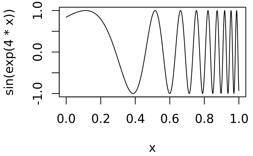
In this code, x is a pronoun: it doesn’t represent a single concrete value, but is instead a placeholder that varies over the range of the plot. One way to implement curve() is to turn that expression into a function with a single argument, x, then call that function:
curve2 <- function(expr, xlim = c(0, 1), n = 100) {
  expr <- enexpr(expr)
  f <- new_function(exprs(x = ), expr)

  x <- seq(xlim[1], xlim[2], length = n)
  y <- f(x)

  plot(x, y, type = "l", ylab = expr_text(expr))
}
curve2(sin(exp(4 * x)), n = 1000)
Functions like curve() that use an expression containing a pronoun are known as anaphoric functions72.
19.7.5 Exercises
In the linear-model example, we could replace the
expr()inreduce(summands, ~ expr(!!.x + !!.y))withcall2():reduce(summands, call2, "+"). Compare and contrast the two approaches. Which do you think is easier to read?Re-implement the Box-Cox transform defined below using unquoting and
new_function():bc <- function(lambda) { if (lambda == 0) { function(x) log(x) } else { function(x) (x ^ lambda - 1) / lambda } }Re-implement the simple
compose()defined below using quasiquotation andnew_function():compose <- function(f, g) { function(...) f(g(...)) }