10.2 Factory fundamentals

The key idea that makes function factories work can be expressed very concisely:

The enclosing environment of the manufactured function is an execution environment of the function factory.

It only takes few words to express these big ideas, but it takes a lot more work to really understand what this means. This section will help you put the pieces together with interactive exploration and some diagrams.

10.2.1 Environments

Let’s start by taking a look at square() and cube():

square
#> function(x) {
#>     x ^ exp
#>   }
#> <environment: 0x5582604af8d8>

cube
#> function(x) {
#>     x ^ exp
#>   }
#> <bytecode: 0x558261e8c8d0>
#> <environment: 0x558260998060>

It’s obvious where x comes from, but how does R find the value associated with exp? Simply printing the manufactured functions is not revealing because the bodies are identical; the contents of the enclosing environment are the important factors. We can get a little more insight by using rlang::env_print(). That shows us that we have two different environments (each of which was originally an execution environment of power1()). The environments have the same parent, which is the enclosing environment of power1(), the global environment.

env_print(square)
#> <environment: 0x5582604af8d8>
#> parent: <environment: global>
#> bindings:
#>  * exp: <dbl>

env_print(cube)
#> <environment: 0x558260998060>
#> parent: <environment: global>
#> bindings:
#>  * exp: <dbl>

env_print() shows us that both environments have a binding to exp, but we want to see its value⁴¹. We can do that by first getting the environment of the function, and then extracting the values:

fn_env(square)$exp
#> [1] 2

fn_env(cube)$exp
#> [1] 3

This is what makes manufactured functions behave differently from one another: names in the enclosing environment are bound to different values.

10.2.2 Diagram conventions

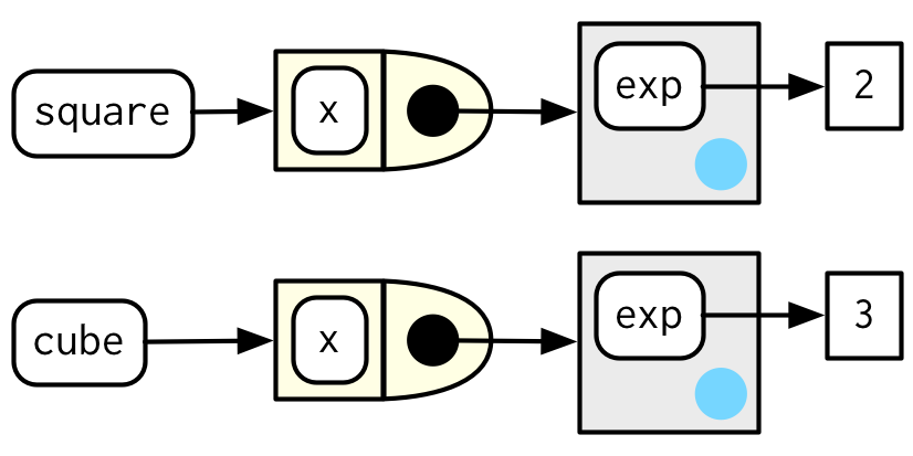
We can also show these relationships in a diagram:

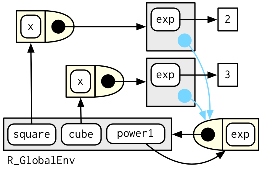
There’s a lot going on this diagram and some of the details aren’t that important. We can simplify considerably by using two conventions:

Any free floating symbol lives in the global environment.
Any environment without an explicit parent inherits from the global environment.

This view, which focuses on the environments, doesn’t show any direct link between cube() and square(). That’s because the link is the through the body of the function, which is identical for both, but is not shown in this diagram.

To finish up, let’s look at the execution environment of square(10). When square() executes x ^ exp it finds x in the execution environment and exp in its enclosing environment.

square(10)
#> [1] 100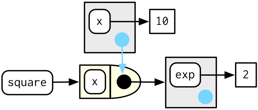

10.2.3 Forcing evaluation

There’s a subtle bug in power1() caused by lazy evaluation. To see the problem we need to introduce some indirection:

x <- 2
square <- power1(x)
x <- 3

What should square(2) return? You would hope it returns 4:

square(2)
#> [1] 8

Unfortunately it doesn’t because x is only evaluated lazily when square() is run, not when power1() is run. In general, this problem will arise whenever a binding changes in between calling the factory function and calling the manufactured function. This is likely to only happen rarely, but when it does, it will lead to a real head-scratcher of a bug.

We can fix this problem by forcing evaluation with force():

power2 <- function(exp) {
  force(exp)
  function(x) {
    x ^ exp
  }
}

x <- 2
square <- power2(x)
x <- 3
square(2)
#> [1] 4

Whenever you create a function factory, make sure every argument is evaluated, using force() as necessary if the argument is only used by the manufactured function.

10.2.4 Stateful functions

Function factories also allow you to maintain state across function invocations, which is generally hard to do because of the fresh start principle described in Section 6.4.3.

There are two things that make this possible:

The enclosing environment of the manufactured function is unique and constant.
R has a special assignment operator, <<-, which modifies bindings in the enclosing environment.

The usual assignment operator, <-, always creates a binding in the current environment. The super assignment operator, <<- rebinds an existing name found in a parent environment.

The following example shows how we can combine these ideas to create a function that records how many times it has been called:

new_counter <- function() {
  i <- 0
  
  function() {
    i <<- i + 1
    i
  }
}

counter_one <- new_counter()
counter_two <- new_counter()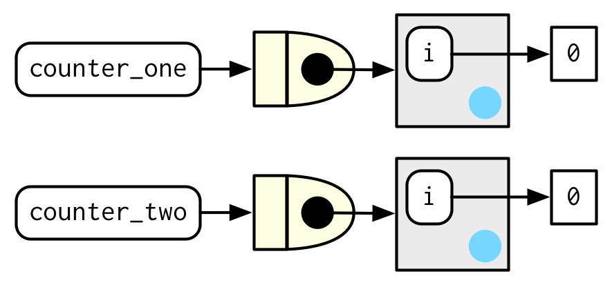

When the manufactured function is run i <<- i + 1 will modify i in its enclosing environment. Because manufactured functions have independent enclosing environments, they have independent counts:

counter_one()
#> [1] 1
counter_one()
#> [1] 2
counter_two()
#> [1] 1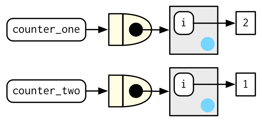

Stateful functions are best used in moderation. As soon as your function starts managing the state of multiple variables, it’s better to switch to R6, the topic of Chapter 14.

10.2.5 Garbage collection

With most functions, you can rely on the garbage collector to clean up any large temporary objects created inside a function. However, manufactured functions hold on to the execution environment, so you’ll need to explicitly unbind any large temporary objects with rm(). Compare the sizes of g1() and g2() in the example below:

f1 <- function(n) {
  x <- runif(n)
  m <- mean(x)
  function() m
}

g1 <- f1(1e6)
lobstr::obj_size(g1)
#> 8,013,080 B

f2 <- function(n) {
  x <- runif(n)
  m <- mean(x)
  rm(x)
  function() m
}

g2 <- f2(1e6)
lobstr::obj_size(g2)
#> 12,920 B

10.2.6 Exercises

The definition of force() is simple:

force
#> function (x) 
#> x
#> <bytecode: 0x55825fd82930>
#> <environment: namespace:base>

Why is it better to force(x) instead of just x?

Base R contains two function factories, approxfun() and ecdf(). Read their documentation and experiment to figure out what the functions do and what they return.

Create a function pick() that takes an index, i, as an argument and returns a function with an argument x that subsets x with i.

pick(1)(x)
# should be equivalent to
x[[1]]

lapply(mtcars, pick(5))
# should be equivalent to
lapply(mtcars, function(x) x[[5]])

Create a function that creates functions that compute the i^th central moment of a numeric vector. You can test it by running the following code:
```
m1 <- moment(1)
m2 <- moment(2)

x <- runif(100)
stopifnot(all.equal(m1(x), 0))
stopifnot(all.equal(m2(x), var(x) * 99 / 100))
```
What happens if you don’t use a closure? Make predictions, then verify with the code below.
```
i <- 0
new_counter2 <- function() {
  i <<- i + 1
  i
}
```

What happens if you use <- instead of <<-? Make predictions, then verify with the code below.

new_counter3 <- function() {
  i <- 0
  function() {
    i <- i + 1
    i
  }
}

A future version of env_print() is likely to do better at summarising the contents so you don’t need this step.↩︎