10.3 Graphical factories
We’ll begin our exploration of useful function factories with a few examples from ggplot2.
10.3.1 Labelling
One of the goals of the scales package is to make it easy to customise the labels on ggplot2. It provides many functions to control the fine details of axes and legends. The formatter functions42 are a useful class of functions which make it easier to control the appearance of axis breaks. The design of these functions might initially seem a little odd: they all return a function, which you have to call in order to format a number.
y <- c(12345, 123456, 1234567)
comma_format()(y)
#> [1] "12,345"    "123,456"   "1,234,567"

number_format(scale = 1e-3, suffix = " K")(y)
#> [1] "12 K"    "123 K"   "1 235 K"
In other words, the primary interface is a function factory. At first glance, this seems to add extra complexity for little gain. But it enables a nice interaction with ggplot2’s scales, because they accept functions in the label argument:
df <- data.frame(x = 1, y = y)
core <- ggplot(df, aes(x, y)) +
geom_point() +
scale_x_continuous(breaks = 1, labels = NULL) +
labs(x = NULL, y = NULL)
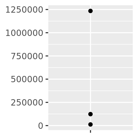
core
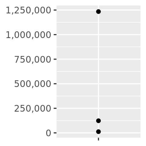
core + scale_y_continuous(
labels = comma_format()
)
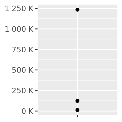
core + scale_y_continuous(
labels = number_format(scale = 1e-3, suffix = " K")
)
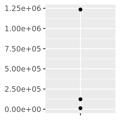
core + scale_y_continuous(
labels = scientific_format()
)
10.3.2 Histogram bins
A little known feature of geom_histogram() is that the binwidth argument can be a function. This is particularly useful because the function is executed once for each group, which means you can have different binwidths in different facets, which is otherwise not possible.
To illustrate this idea, and see where variable binwidth might be useful, I’m going to construct an example where a fixed binwidth isn’t great.
# construct some sample data with very different numbers in each cell
sd <- c(1, 5, 15)
n <- 100

df <- data.frame(x = rnorm(3 * n, sd = sd), sd = rep(sd, n))

ggplot(df, aes(x)) +
  geom_histogram(binwidth = 2) +
  facet_wrap(~ sd, scales = "free_x") +
  labs(x = NULL)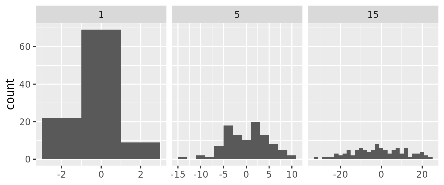
Here each facet has the same number of observations, but the variability is very different. It would be nice if we could request that the binwidths vary so we get approximately the same number of observations in each bin. One way to do that is with a function factory that inputs the desired number of bins (n), and outputs a function that takes a numeric vector and returns a binwidth:
binwidth_bins <- function(n) {
  force(n)

  function(x) {
    (max(x) - min(x)) / n
  }
}

ggplot(df, aes(x)) +
  geom_histogram(binwidth = binwidth_bins(20)) +
  facet_wrap(~ sd, scales = "free_x") +
  labs(x = NULL)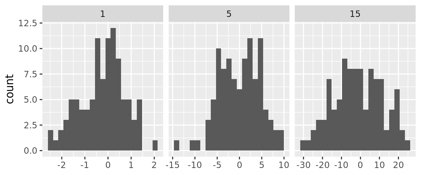
We could use this same pattern to wrap around the base R functions that automatically find the so-called optimal43 binwidth, nclass.Sturges(), nclass.scott(), and nclass.FD():
base_bins <- function(type) {
  fun <- switch(type,
    Sturges = nclass.Sturges,
    scott = nclass.scott,
    FD = nclass.FD,
    stop("Unknown type", call. = FALSE)
  )

  function(x) {
    (max(x) - min(x)) / fun(x)
  }
}

ggplot(df, aes(x)) +
  geom_histogram(binwidth = base_bins("FD")) +
  facet_wrap(~ sd, scales = "free_x") +
  labs(x = NULL)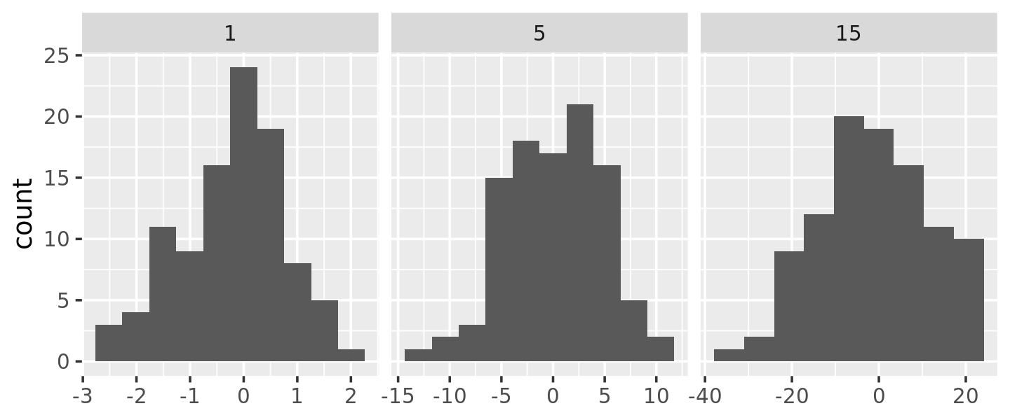
10.3.3 ggsave()
Finally, I want to show a function factory used internally by ggplot2. ggplot2:::plot_dev() is used by ggsave() to go from a file extension (e.g. png, jpeg etc) to a graphics device function (e.g. png(), jpeg()). The challenge here arises because the base graphics devices have some minor inconsistencies which we need to paper over:
Most have
filenameas first argument but some havefile.The
widthandheightof raster graphic devices use pixels units by default, but the vector graphics use inches.
A mildly simplified version of plot_dev() is shown below:
plot_dev <- function(ext, dpi = 96) {
  force(dpi)

  switch(ext,
    eps =  ,
    ps  =  function(path, ...) {
      grDevices::postscript(
        file = filename, ..., onefile = FALSE,
        horizontal = FALSE, paper = "special"
      )
    },
    pdf = function(filename, ...) grDevices::pdf(file = filename, ...),
    svg = function(filename, ...) svglite::svglite(file = filename, ...),
    emf = ,
    wmf = function(...) grDevices::win.metafile(...),
    png = function(...) grDevices::png(..., res = dpi, units = "in"),
    jpg = ,
    jpeg = function(...) grDevices::jpeg(..., res = dpi, units = "in"),
    bmp = function(...) grDevices::bmp(..., res = dpi, units = "in"),
    tiff = function(...) grDevices::tiff(..., res = dpi, units = "in"),
    stop("Unknown graphics extension: ", ext, call. = FALSE)
  )
}

plot_dev("pdf")
#> function(filename, ...) grDevices::pdf(file = filename, ...)
#> <bytecode: 0x558263cb2d40>
#> <environment: 0x558262c0f808>
plot_dev("png")
#> function(...) grDevices::png(..., res = dpi, units = "in")
#> <bytecode: 0x558263e861e8>
#> <environment: 0x55826423d380>
10.3.4 Exercises
- Compare and contrast
ggplot2::label_bquote()withscales::number_format()
It’s an unfortunate accident of history that scales uses function suffixes instead of function prefixes. That’s because it was written before I understood the autocomplete advantages to using common prefixes instead of common suffixes.↩︎
ggplot2 doesn’t expose these functions directly because I don’t think the definition of optimality needed to make the problem mathematically tractable is a good match to the actual needs of data exploration.↩︎