9.4 Map variants
There are 23 primary variants of map(). So far, you’ve learned about five (map(), map_lgl(), map_int(), map_dbl() and map_chr()). That means that you’ve got 18 (!!) more to learn. That sounds like a lot, but fortunately the design of purrr means that you only need to learn five new ideas:
- Output same type as input with
modify() - Iterate over two inputs with
map2(). - Iterate with an index using
imap() - Return nothing with
walk(). - Iterate over any number of inputs with
pmap().
The map family of functions has orthogonal input and outputs, meaning that we can organise all the family into a matrix, with inputs in the rows and outputs in the columns. Once you’ve mastered the idea in a row, you can combine it with any column; once you’ve mastered the idea in a column, you can combine it with any row. That relationship is summarised in the following table:
| List | Atomic | Same type | Nothing | |
|---|---|---|---|---|
| One argument | map() |
map_lgl(), … |
modify() |
walk() |
| Two arguments | map2() |
map2_lgl(), … |
modify2() |
walk2() |
| One argument + index | imap() |
imap_lgl(), … |
imodify() |
iwalk() |
| N arguments | pmap() |
pmap_lgl(), … |
— | pwalk() |
9.4.1 Same type of output as input: modify()
Imagine you wanted to double every column in a data frame. You might first try using map(), but map() always returns a list:
df <- data.frame(
  x = 1:3,
  y = 6:4
)

map(df, ~ .x * 2)
#> $x
#> [1] 2 4 6
#>
#> $y
#> [1] 12 10  8
If you want to keep the output as a data frame, you can use modify(), which always returns the same type of output as the input:
modify(df, ~ .x * 2)
#>   x  y
#> 1 2 12
#> 2 4 10
#> 3 6  8
Despite the name, modify() doesn’t modify in place, it returns a modified copy, so if you wanted to permanently modify df, you’d need to assign it:
df <- modify(df, ~ .x * 2)As usual, the basic implementation of modify() is simple, and in fact it’s even simpler than map() because we don’t need to create a new output vector; we can just progressively replace the input. (The real code is a little complex to handle edge cases more gracefully.)
simple_modify <- function(x, f, ...) {
  for (i in seq_along(x)) {
    x[[i]] <- f(x[[i]], ...)
  }
  x
}
In Section 9.6.2 you’ll learn about a very useful variant of modify(), called modify_if(). This allows you to (e.g.) only double numeric columns of a data frame with modify_if(df, is.numeric, ~ .x * 2).
9.4.2 Two inputs: map2() and friends
map() is vectorised over a single argument, .x. This means it only varies .x when calling .f, and all other arguments are passed along unchanged, thus making it poorly suited for some problems. For example, how would you find a weighted mean when you have a list of observations and a list of weights? Imagine we have the following data:
xs <- map(1:8, ~ runif(10))
xs[[1]][[1]] <- NA
ws <- map(1:8, ~ rpois(10, 5) + 1)
You can use map_dbl() to compute the unweighted means:
map_dbl(xs, mean)
#> [1]    NA 0.463 0.551 0.453 0.564 0.501 0.371 0.443
But passing ws as an additional argument doesn’t work because arguments after .f are not transformed:
map_dbl(xs, weighted.mean, w = ws)
#> Error in weighted.mean.default(.x[[i]], ...): 'x' and 'w' must have the same
#> length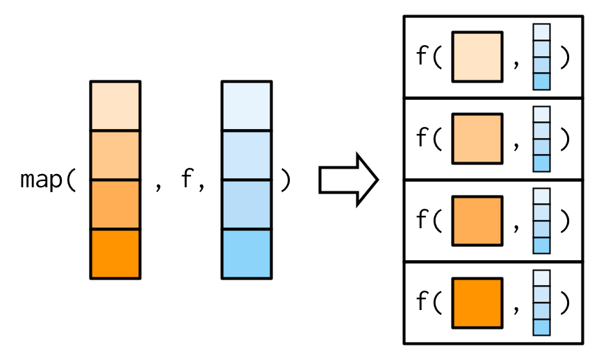
We need a new tool: a map2(), which is vectorised over two arguments. This means both .x and .y are varied in each call to .f:
map2_dbl(xs, ws, weighted.mean)
#> [1]    NA 0.451 0.603 0.452 0.563 0.510 0.342 0.464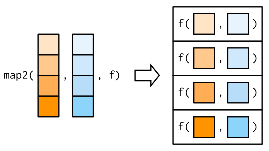
The arguments to map2() are slightly different to the arguments to map() as two vectors come before the function, rather than one. Additional arguments still go afterwards:
map2_dbl(xs, ws, weighted.mean, na.rm = TRUE)
#> [1] 0.504 0.451 0.603 0.452 0.563 0.510 0.342 0.464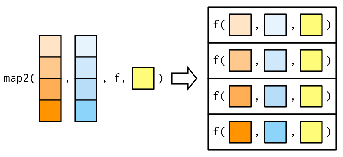
The basic implementation of map2() is simple, and quite similar to that of map(). Instead of iterating over one vector, we iterate over two in parallel:
simple_map2 <- function(x, y, f, ...) {
  out <- vector("list", length(x))
  for (i in seq_along(x)) {
    out[[i]] <- f(x[[i]], y[[i]], ...)
  }
  out
}
One of the big differences between map2() and the simple function above is that map2() recycles its inputs to make sure that they’re the same length:
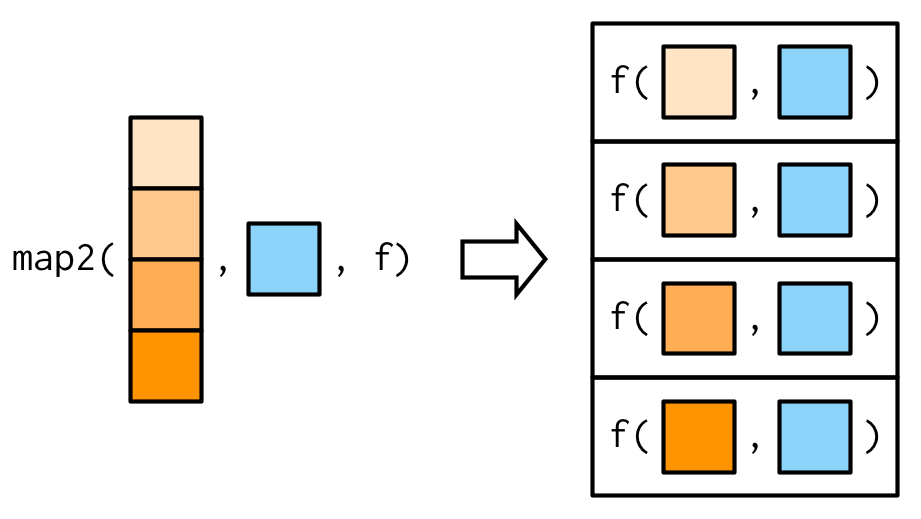
In other words, map2(x, y, f) will automatically behave like map(x, f, y) when needed. This is helpful when writing functions; in scripts you’d generally just use the simpler form directly.
The closest base equivalent to map2() is Map(), which is discussed in Section 9.4.5.
9.4.3 No outputs: walk() and friends
Most functions are called for the value that they return, so it makes sense to capture and store the value with a map() function. But some functions are called primarily for their side-effects (e.g. cat(), write.csv(), or ggsave()) and it doesn’t make sense to capture their results. Take this simple example that displays a welcome message using cat(). cat() returns NULL, so while map() works (in the sense that it generates the desired welcomes), it also returns list(NULL, NULL).
welcome <- function(x) {
  cat("Welcome ", x, "!\n", sep = "")
}
names <- c("Hadley", "Jenny")

# As well as generate the welcomes, it also shows
# the return value of cat()
map(names, welcome)
#> Welcome Hadley!
#> Welcome Jenny!
#> [[1]]
#> NULL
#>
#> [[2]]
#> NULL
You could avoid this problem by assigning the results of map() to a variable that you never use, but that would muddy the intent of the code. Instead, purrr provides the walk family of functions that ignore the return values of the .f and instead return .x invisibly40.
walk(names, welcome)
#> Welcome Hadley!
#> Welcome Jenny!
My visual depiction of walk attempts to capture the important difference from map(): the outputs are ephemeral, and the input is returned invisibly.
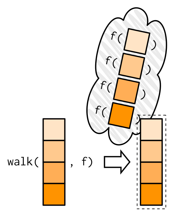
One of the most useful walk() variants is walk2() because a very common side-effect is saving something to disk, and when saving something to disk you always have a pair of values: the object and the path that you want to save it to.
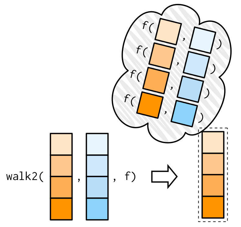
For example, imagine you have a list of data frames (which I’ve created here using split()), and you’d like to save each one to a separate CSV file. That’s easy with walk2():
temp <- tempfile()
dir.create(temp)

cyls <- split(mtcars, mtcars$cyl)
paths <- file.path(temp, paste0("cyl-", names(cyls), ".csv"))
walk2(cyls, paths, write.csv)

dir(temp)
#> [1] "cyl-4.csv" "cyl-6.csv" "cyl-8.csv"
Here the walk2() is equivalent to write.csv(cyls[[1]], paths[[1]]), write.csv(cyls[[2]], paths[[2]]), write.csv(cyls[[3]], paths[[3]]).
There is no base equivalent to walk(); either wrap the result of lapply() in invisible() or save it to a variable that is never used.
9.4.4 Iterating over values and indices
There are three basic ways to loop over a vector with a for loop:
- Loop over the elements:
for (x in xs) - Loop over the numeric indices:
for (i in seq_along(xs)) - Loop over the names:
for (nm in names(xs))
The first form is analogous to the map() family. The second and third forms are equivalent to the imap() family which allows you to iterate over the values and the indices of a vector in parallel.
imap() is like map2() in the sense that your .f gets called with two arguments, but here both are derived from the vector. imap(x, f) is equivalent to map2(x, names(x), f) if x has names, and map2(x, seq_along(x), f) if it does not.
imap() is often useful for constructing labels:
imap_chr(iris, ~ paste0("The first value of ", .y, " is ", .x[[1]]))
#>                             Sepal.Length
#> "The first value of Sepal.Length is 5.1"
#>                              Sepal.Width
#>  "The first value of Sepal.Width is 3.5"
#>                             Petal.Length
#> "The first value of Petal.Length is 1.4"
#>                              Petal.Width
#>  "The first value of Petal.Width is 0.2"
#>                                  Species
#>   "The first value of Species is setosa"
If the vector is unnamed, the second argument will be the index:
x <- map(1:6, ~ sample(1000, 10))
imap_chr(x, ~ paste0("The highest value of ", .y, " is ", max(.x)))
#> [1] "The highest value of 1 is 975" "The highest value of 2 is 915"
#> [3] "The highest value of 3 is 982" "The highest value of 4 is 955"
#> [5] "The highest value of 5 is 971" "The highest value of 6 is 696"
imap() is a useful helper if you want to work with the values in a vector along with their positions.
9.4.5 Any number of inputs: pmap() and friends
Since we have map() and map2(), you might expect map3(), map4(), map5(), … But where would you stop? Instead of generalising map2() to an arbitrary number of arguments, purrr takes a slightly different tack with pmap(): you supply it a single list, which contains any number of arguments. In most cases, that will be a list of equal-length vectors, i.e. something very similar to a data frame. In diagrams, I’ll emphasise that relationship by drawing the input similar to a data frame.
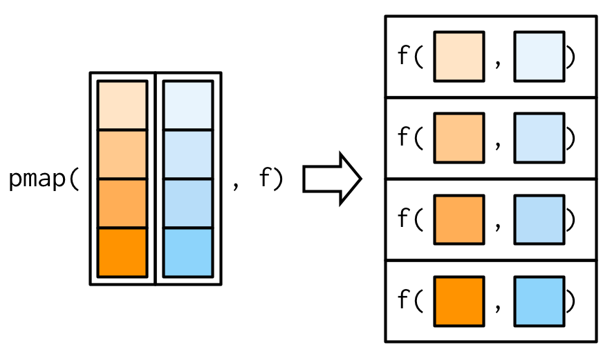
There’s a simple equivalence between map2() and pmap(): map2(x, y, f) is the same as pmap(list(x, y), f). The pmap() equivalent to the map2_dbl(xs, ws, weighted.mean) used above is:
pmap_dbl(list(xs, ws), weighted.mean)
#> [1]    NA 0.451 0.603 0.452 0.563 0.510 0.342 0.464
As before, the varying arguments come before .f (although now they must be wrapped in a list), and the constant arguments come afterwards.
pmap_dbl(list(xs, ws), weighted.mean, na.rm = TRUE)
#> [1] 0.504 0.451 0.603 0.452 0.563 0.510 0.342 0.464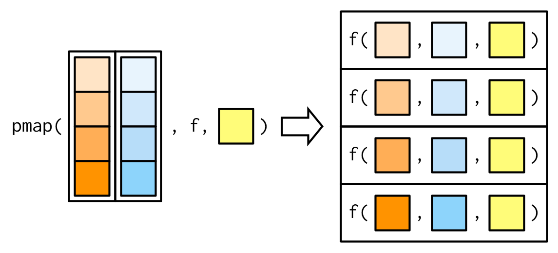
A big difference between pmap() and the other map functions is that pmap() gives you much finer control over argument matching because you can name the components of the list. Returning to our example from Section 9.2.5, where we wanted to vary the trim argument to x, we could instead use pmap():
trims <- c(0, 0.1, 0.2, 0.5)
x <- rcauchy(1000)

pmap_dbl(list(trim = trims), mean, x = x)
#> [1] -6.6740  0.0210  0.0235  0.0151
I think it’s good practice to name the components of the list to make it very clear how the function will be called.
It’s often convenient to call pmap() with a data frame. A handy way to create that data frame is with tibble::tribble(), which allows you to describe a data frame row-by-row (rather than column-by-column, as usual): thinking about the parameters to a function as a data frame is a very powerful pattern. The following example shows how you might draw random uniform numbers with varying parameters:
params <- tibble::tribble(
~ n, ~ min, ~ max,
1L, 0, 1,
2L, 10, 100,
3L, 100, 1000
)
pmap(params, runif)
#> [[1]]
#> [1] 0.332
#>
#> [[2]]
#> [1] 53.5 47.6
#>
#> [[3]]
#> [1] 231 715 515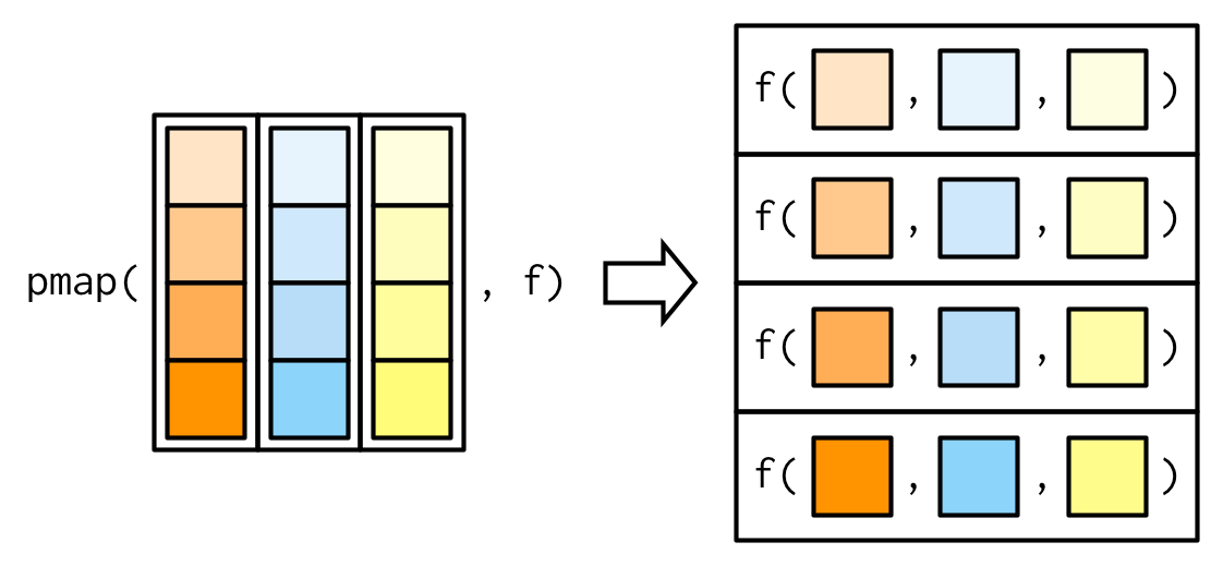 Here, the column names are critical: I’ve carefully chosen to match them to the arguments to
 runif(), so the pmap(params, runif) is equivalent to runif(n = 1L, min = 0, max = 1), runif(n = 2, min = 10, max = 100), runif(n = 3L, min = 100, max = 1000). (If you have a data frame in hand, and the names don’t match, use dplyr::rename() or similar.)
There are two base equivalents to the pmap() family: Map() and mapply(). Both have significant drawbacks:
Map()vectorises over all arguments so you cannot supply arguments that do not vary.mapply()is the multidimensional version ofsapply(); conceptually it takes the output ofMap()and simplifies it if possible. This gives it similar issues tosapply(). There is no multi-input equivalent ofvapply().
9.4.6 Exercises
Explain the results of
modify(mtcars, 1).Rewrite the following code to use
iwalk()instead ofwalk2(). What are the advantages and disadvantages?cyls <- split(mtcars, mtcars$cyl) paths <- file.path(temp, paste0("cyl-", names(cyls), ".csv")) walk2(cyls, paths, write.csv)Explain how the following code transforms a data frame using functions stored in a list.
trans <- list(
  disp = function(x) x * 0.0163871,
  am = function(x) factor(x, labels = c("auto", "manual"))
)

nm <- names(trans)
mtcars[nm] <- map2(trans, mtcars[nm], function(f, var) f(var))
Compare and contrast the
map2()approach to thismap()approach:mtcars[vars] <- map(vars, ~ trans[[.x]](mtcars[[.x]]))What does
write.csv()return? i.e. what happens if you use it withmap2()instead ofwalk2()?