23.2 Profiling

Across programming languages, the primary tool used to understand code performance is the profiler. There are a number of different types of profilers, but R uses a fairly simple type called a sampling or statistical profiler. A sampling profiler stops the execution of code every few milliseconds and records the call stack (i.e. which function is currently executing, and the function that called the function, and so on). For example, consider f(), below:

f <- function() {
  pause(0.1)
  g()
  h()
}
g <- function() {
  pause(0.1)
  h()
}
h <- function() {
  pause(0.1)
}

(I use profvis::pause() instead of Sys.sleep() because Sys.sleep() does not appear in profiling outputs because as far as R can tell, it doesn’t use up any computing time.)

If we profiled the execution of f(), stopping the execution of code every 0.1 s, we’d see a profile like this:

"pause" "f" 
"pause" "g" "f"
"pause" "h" "g" "f"
"pause" "h" "f"

Each line represents one “tick” of the profiler (0.1 s in this case), and function calls are recorded from right to left: the first line shows f() calling pause(). It shows that the code spends 0.1 s running f(), then 0.2 s running g(), then 0.1 s running h().

If we actually profile f(), using utils::Rprof() as in the code below, we’re unlikely to get such a clear result.

tmp <- tempfile()
Rprof(tmp, interval = 0.1)
f()
Rprof(NULL)
writeLines(readLines(tmp))
#> sample.interval=100000
#> "pause" "g" "f" 
#> "pause" "h" "g" "f" 
#> "pause" "h" "f" 

That’s because all profilers must make a fundamental trade-off between accuracy and performance. The compromise that makes, using a sampling profiler, only has minimal impact on performance, but is fundamentally stochastic because there’s some variability in both the accuracy of the timer and in the time taken by each operation. That means each time that you profile you’ll get a slightly different answer. Fortunately, the variability most affects functions that take very little time to run, which are also the functions of least interest.

23.2.1 Visualising profiles

The default profiling resolution is quite small, so if your function takes even a few seconds it will generate hundreds of samples. That quickly grows beyond our ability to look at directly, so instead of using utils::Rprof() we’ll use the profvis package to visualise aggregates. profvis also connects profiling data back to the underlying source code, making it easier to build up a mental model of what you need to change. If you find profvis doesn’t help for your code, you might try one of the other options like utils::summaryRprof() or the proftools package (Tierney and Jarjour 2016).

There are two ways to use profvis:

• From the Profile menu in RStudio.

• With profvis::profvis(). I recommend storing your code in a separate file and source()ing it in; this will ensure you get the best connection between profiling data and source code.

  source("profiling-example.R")
  profvis(f())

After profiling is complete, profvis will open an interactive HTML document that allows you to explore the results. There are two panes, as shown in Figure 23.1.

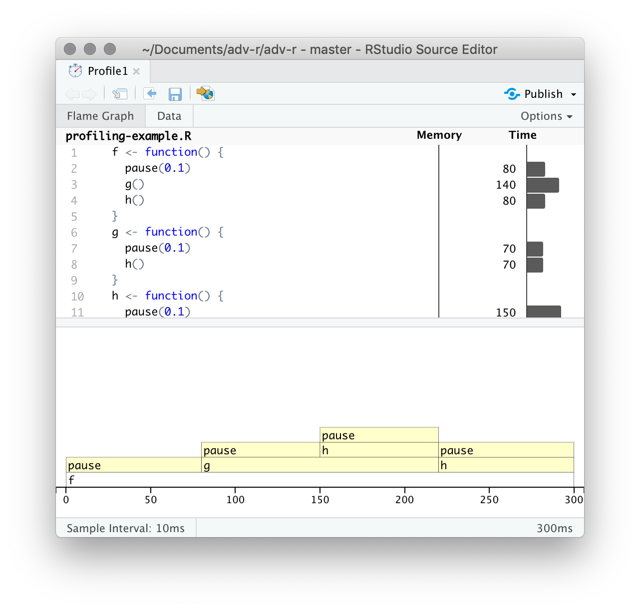
Figure 23.1: profvis output showing source on top and flame graph below.

The top pane shows the source code, overlaid with bar graphs for memory and execution time for each line of code. Here I’ll focus on time, and we’ll come back to memory shortly. This display gives you a good overall feel for the bottlenecks but doesn’t always help you precisely identify the cause. Here, for example, you can see that h() takes 150 ms, twice as long as g(); that’s not because the function is slower, but because it’s called twice as often.

The bottom pane displays a flame graph showing the full call stack. This allows you to see the full sequence of calls leading to each function, allowing you to see that h() is called from two different places. In this display you can mouse over individual calls to get more information, and see the corresponding line of source code, as in Figure 23.2.

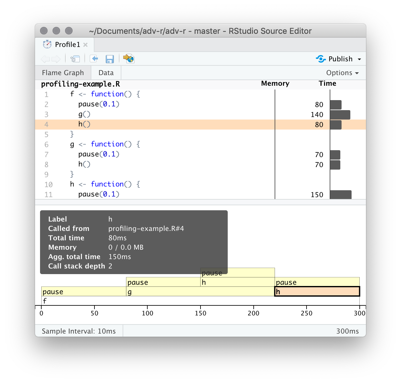
Figure 23.2: Hovering over a call in the flamegraph highlights the corresponding line of code, and displays additional information about performance.

Alternatively, you can use the data tab, Figure 23.3 lets you interactively dive into the tree of performance data. This is basically the same display as the flame graph (rotated 90 degrees), but it’s more useful when you have very large or deeply nested call stacks because you can choose to interactively zoom into only selected components.

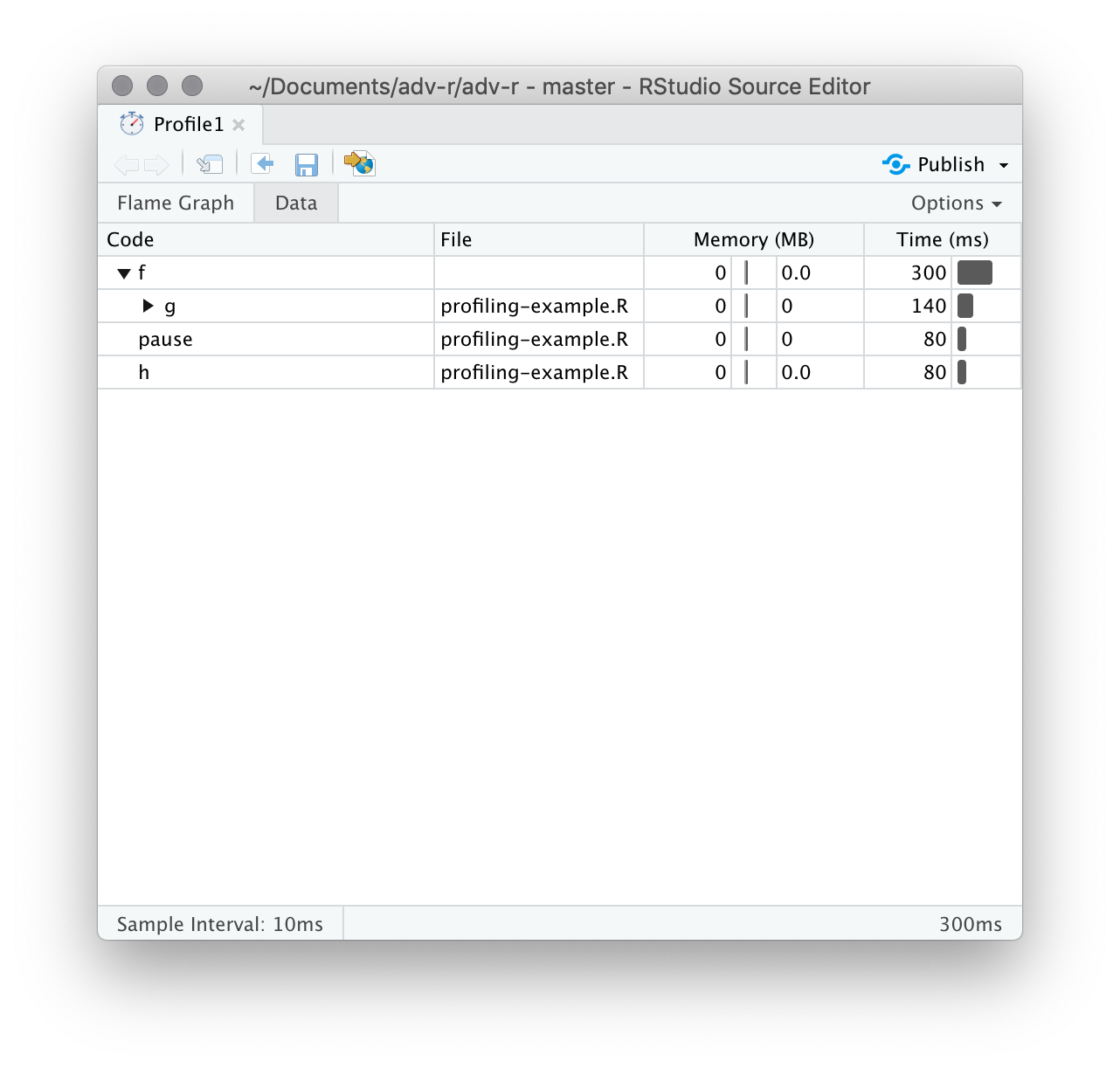
Figure 23.3: The data gives an interactive tree that allows you to selectively zoom into key components

23.2.2 Memory profiling

There is a special entry in the flame graph that doesn’t correspond to your code: <GC>, which indicates that the garbage collector is running. If <GC> is taking a lot of time, it’s usually an indication that you’re creating many short-lived objects. For example, take this small snippet of code:

x <- integer()
for (i in 1:1e4) {
  x <- c(x, i)
}

If you profile it, you’ll see that most of the time is spent in the garbage collector, Figure 23.4.

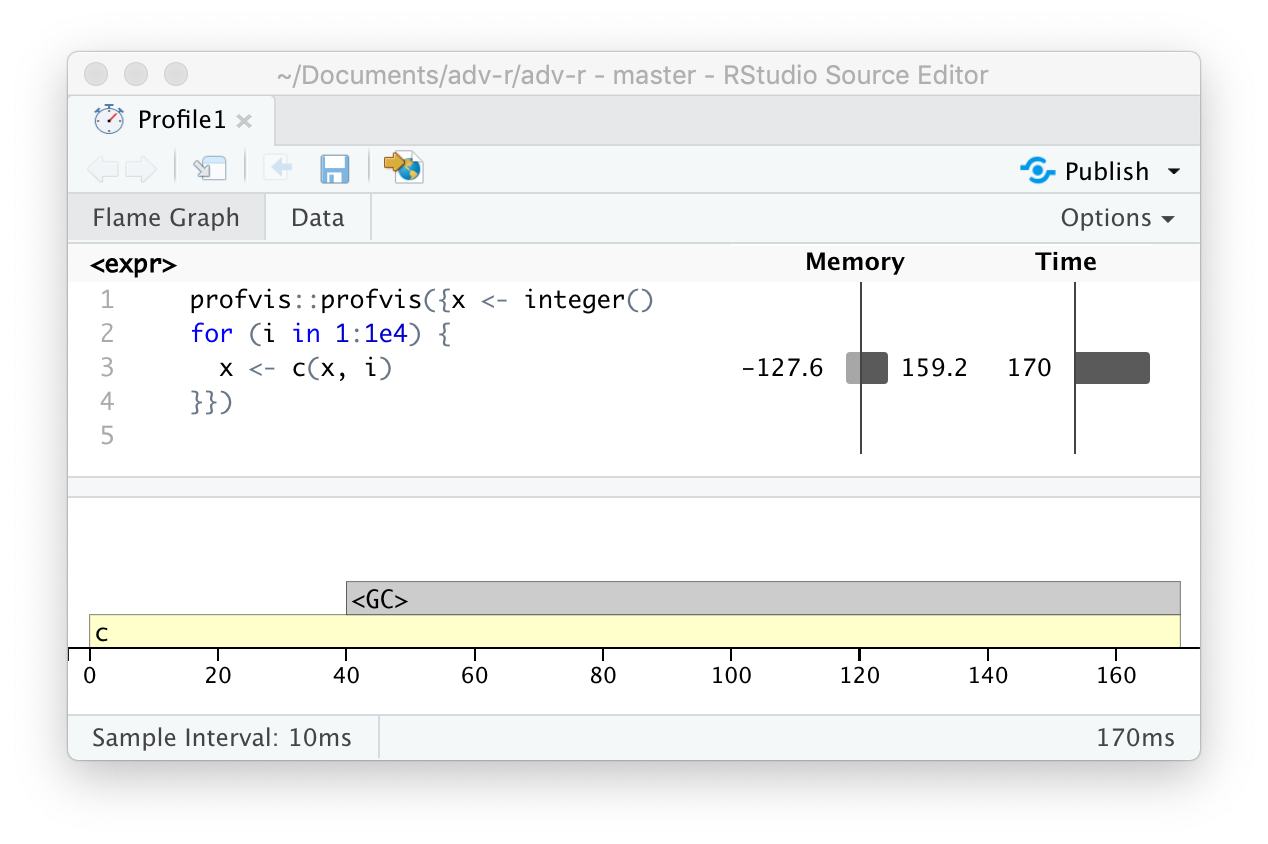
Figure 23.4: Profiling a loop that modifies an existing variable reveals that most time is spent in the garbage collector ().

When you see the garbage collector taking up a lot of time in your own code, you can often figure out the source of the problem by looking at the memory column: you’ll see a line where large amounts of memory are being allocated (the bar on the right) and freed (the bar on the left). Here the problem arises because of copy-on-modify (Section 2.3): each iteration of the loop creates another copy of x. You’ll learn strategies to resolve this type of problem in Section 24.6.

23.2.3 Limitations

There are some other limitations to profiling:

• Profiling does not extend to C code. You can see if your R code calls C/C++ code but not what functions are called inside of your C/C++ code. Unfortunately, tools for profiling compiled code are beyond the scope of this book; start by looking at https://github.com/r-prof/jointprof.

• If you’re doing a lot of functional programming with anonymous functions, it can be hard to figure out exactly which function is being called. The easiest way to work around this is to name your functions.

• Lazy evaluation means that arguments are often evaluated inside another function, and this complicates the call stack (Section 7.5.2). Unfortunately R’s profiler doesn’t store enough information to disentangle lazy evaluation so that in the following code, profiling would make it seem like i() was called by j() because the argument isn’t evaluated until it’s needed by j().

  i <- function() {
    pause(0.1)
    10
  }
  j <- function(x) {
    x + 10
  }
  j(i())

  If this is confusing, use force() (Section 10.2.3) to force computation to happen earlier.

23.2.4 Exercises

1. Profile the following function with torture = TRUE. What is surprising? Read the source code of rm() to figure out what’s going on.

   f <- function(n = 1e5) {
     x <- rep(1, n)
     rm(x)
   }

References

Tierney, Luke, and Riad Jarjour. 2016. Proftools: Profile Output Processing Tools for R. https://CRAN.R-project.org/package=proftools.