9.5 Reduce family
After the map family, the next most important family of functions is the reduce family. This family is much smaller, with only two main variants, and is used less commonly, but it’s a powerful idea, gives us the opportunity to discuss some useful algebra, and powers the map-reduce framework frequently used for processing very large datasets.
9.5.1 Basics
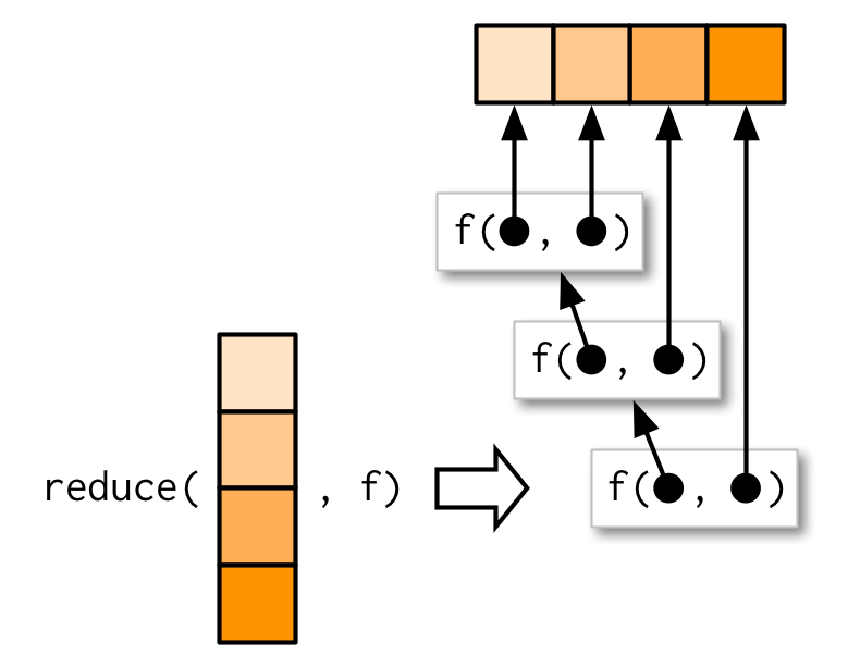
reduce() takes a vector of length n and produces a vector of length 1 by calling a function with a pair of values at a time: reduce(1:4, f) is equivalent to f(f(f(1, 2), 3), 4).
reduce() is a useful way to generalise a function that works with two inputs (a binary function) to work with any number of inputs. Imagine you have a list of numeric vectors, and you want to find the values that occur in every element. First we generate some sample data:
l <- map(1:4, ~ sample(1:10, 15, replace = T))
str(l)
#> List of 4
#>  $ : int [1:15] 7 1 8 8 3 8 2 4 7 10 ...
#>  $ : int [1:15] 3 1 10 2 5 2 9 8 5 4 ...
#>  $ : int [1:15] 6 10 9 5 6 7 8 6 10 8 ...
#>  $ : int [1:15] 9 8 6 4 4 5 2 9 9 6 ...
To solve this challenge we need to use intersect() repeatedly:
out <- l[[1]]
out <- intersect(out, l[[2]])
out <- intersect(out, l[[3]])
out <- intersect(out, l[[4]])
out
#> [1] 8 4
reduce() automates this solution for us, so we can write:
reduce(l, intersect)
#> [1] 8 4
We could apply the same idea if we wanted to list all the elements that appear in at least one entry. All we have to do is switch from intersect() to union():
reduce(l, union)
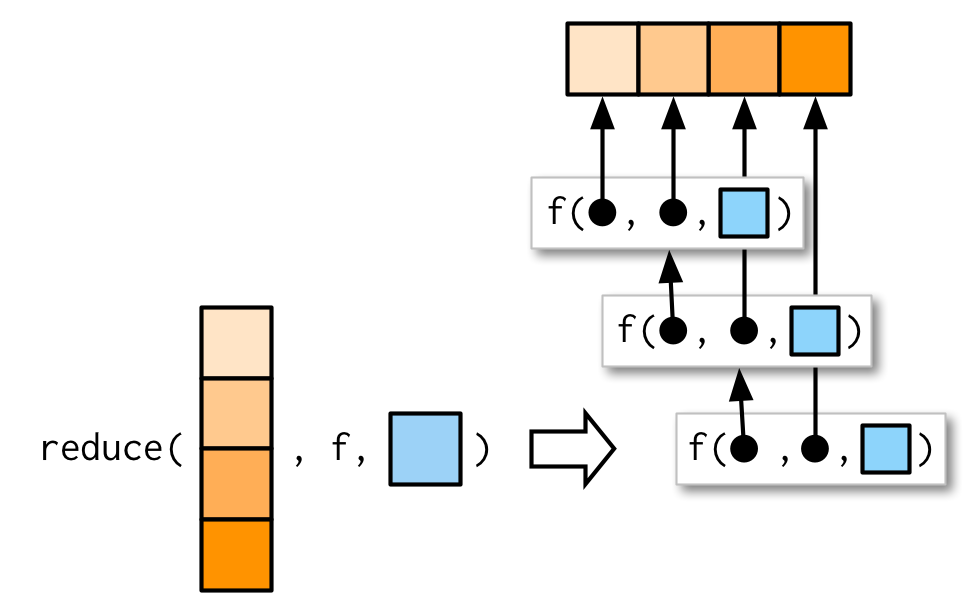
#> [1] 7 1 8 3 2 4 10 5 9 6Like the map family, you can also pass additional arguments. intersect() and union() don’t take extra arguments so I can’t demonstrate them here, but the principle is straightforward and I drew you a picture.
As usual, the essence of reduce() can be reduced to a simple wrapper around a for loop:
simple_reduce <- function(x, f) {
  out <- x[[1]]
  for (i in seq(2, length(x))) {
    out <- f(out, x[[i]])
  }
  out
}
The base equivalent is Reduce(). Note that the argument order is different: the function comes first, followed by the vector, and there is no way to supply additional arguments.
9.5.2 Accumulate
The first reduce() variant, accumulate(), is useful for understanding how reduce works, because instead of returning just the final result, it returns all the intermediate results as well:
accumulate(l, intersect)
#> [[1]]
#>  [1]  7  1  8  8  3  8  2  4  7 10 10  3  7 10 10
#>
#> [[2]]
#> [1]  1  8  3  2  4 10
#>
#> [[3]]
#> [1]  8  4 10
#>
#> [[4]]
#> [1] 8 4
Another useful way to understand reduce is to think about sum(): sum(x) is equivalent to x[[1]] + x[[2]] + x[[3]] + ..., i.e. reduce(x, `+`). Then accumulate(x, `+`) is the cumulative sum:
x <- c(4, 3, 10)
reduce(x, `+`)
#> [1] 17

accumulate(x, `+`)
#> [1]  4  7 17
9.5.3 Output types
In the above example using +, what should reduce() return when x is short, i.e. length 1 or 0? Without additional arguments, reduce() just returns the input when x is length 1:
reduce(1, `+`)
#> [1] 1
This means that reduce() has no way to check that the input is valid:
reduce("a", `+`)
#> [1] "a"
What if it’s length 0? We get an error that suggests we need to use the .init argument:
reduce(integer(), `+`)
#> Error: `.x` is empty, and no `.init` supplied
What should .init be here? To figure that out, we need to see what happens when .init is supplied:
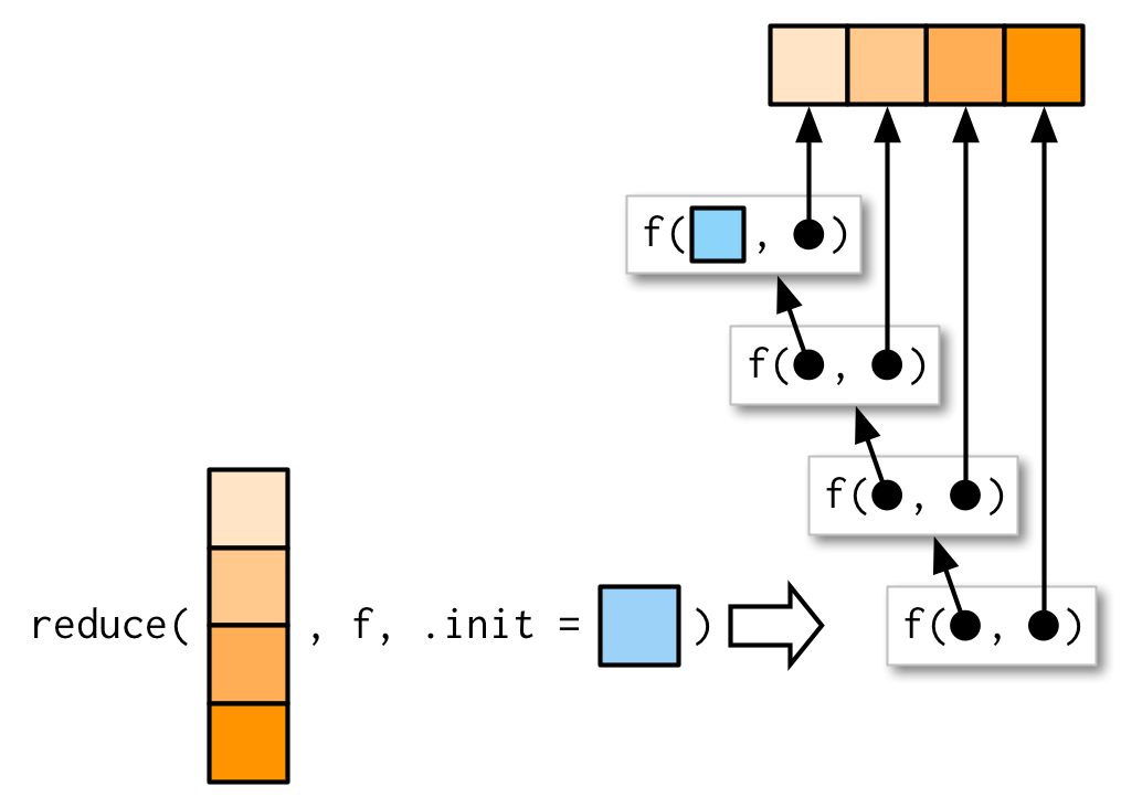
So if we call reduce(1, `+`, init) the result will be 1 + init. Now we know that the result should be just 1, so that suggests that .init should be 0:
reduce(integer(), `+`, .init = 0)
#> [1] 0
This also ensures that reduce() checks that length 1 inputs are valid for the function that you’re calling:
reduce("a", `+`, .init = 0)
#> Error in .x + .y: non-numeric argument to binary operator
If you want to get algebraic about it, 0 is called the identity of the real numbers under the operation of addition: if you add a 0 to any number, you get the same number back. R applies the same principle to determine what a summary function with a zero length input should return:
sum(integer())  # x + 0 = x
#> [1] 0
prod(integer()) # x * 1 = x
#> [1] 1
min(integer())  # min(x, Inf) = x
#> [1] Inf
max(integer())  # max(x, -Inf) = x
#> [1] -Inf
If you’re using reduce() in a function, you should always supply .init. Think carefully about what your function should return when you pass a vector of length 0 or 1, and make sure to test your implementation.
9.5.4 Multiple inputs
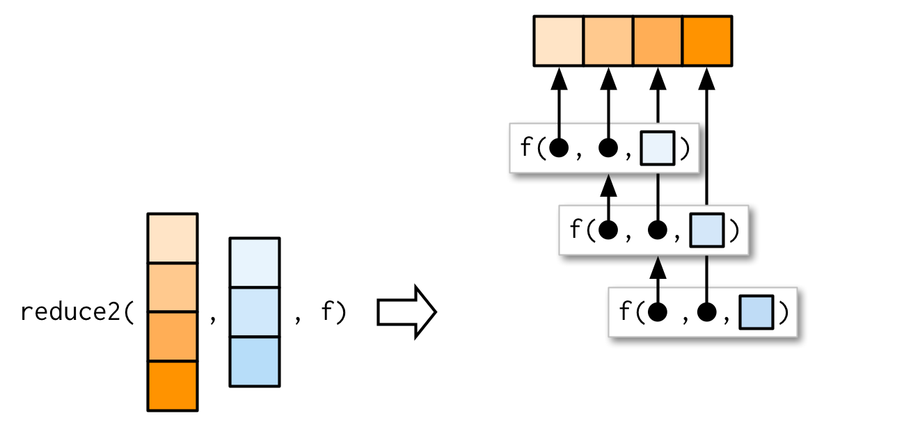
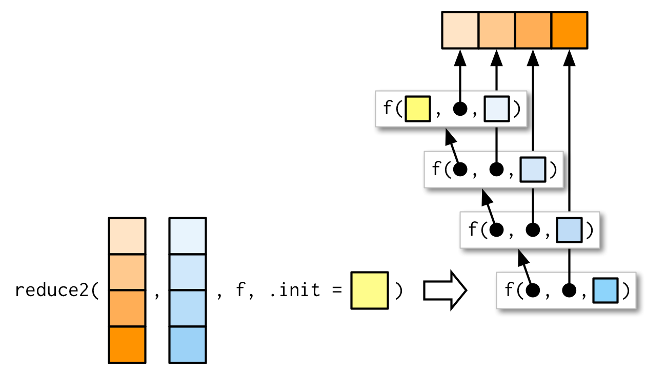
Very occasionally you need to pass two arguments to the function that you’re reducing. For example, you might have a list of data frames that you want to join together, and the variables you use to join will vary from element to element. This is a very specialised scenario, so I don’t want to spend much time on it, but I do want you to know that reduce2() exists.
The length of the second argument varies based on whether or not .init is supplied: if you have four elements of x, f will only be called three times. If you supply init, f will be called four times.
9.5.5 Map-reduce
You might have heard of map-reduce, the idea that powers technology like Hadoop. Now you can see how simple and powerful the underlying idea is: map-reduce is a map combined with a reduce. The difference for large data is that the data is spread over multiple computers. Each computer performs the map on the data that it has, then it sends the result to back to a coordinator which reduces the individual results back to a single result.
As a simple example, imagine computing the mean of a very large vector, so large that it has to be split over multiple computers. You could ask each computer to calculate the sum and the length, and then return those to the coordinator which computes the overall mean by dividing the total sum by the total length.