7.4 Special environments
Most environments are not created by you (e.g. with env()) but are instead created by R. In this section, you’ll learn about the most important environments, starting with the package environments. You’ll then learn about the function environment bound to the function when it is created, and the (usually) ephemeral execution environment created every time the function is called. Finally, you’ll see how the package and function environments interact to support namespaces, which ensure that a package always behaves the same way, regardless of what other packages the user has loaded.
7.4.1 Package environments and the search path
Each package attached by library() or require() becomes one of the parents of the global environment. The immediate parent of the global environment is the last package you attached31, the parent of that package is the second to last package you attached, …
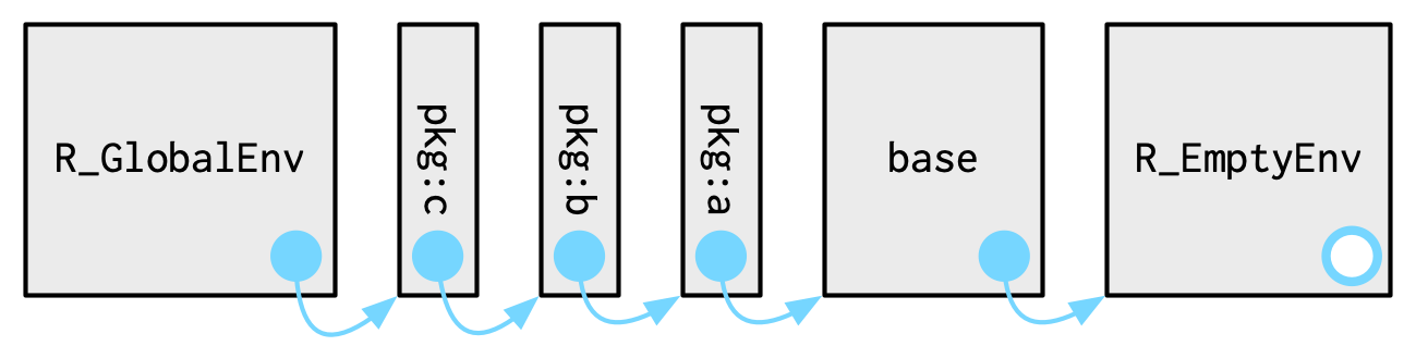
If you follow all the parents back, you see the order in which every package has been attached. This is known as the search path because all objects in these environments can be found from the top-level interactive workspace. You can see the names of these environments with base::search(), or the environments themselves with rlang::search_envs():
search()
#>  [1] ".GlobalEnv"        "package:rlang"     "package:stats"
#>  [4] "package:graphics"  "package:grDevices" "package:utils"
#>  [7] "package:datasets"  "package:methods"   "Autoloads"
#> [10] "package:base"

search_envs()
#>  [[1]] $ <env: global>
#>  [[2]] $ <env: package:rlang>
#>  [[3]] $ <env: package:stats>
#>  [[4]] $ <env: package:graphics>
#>  [[5]] $ <env: package:grDevices>
#>  [[6]] $ <env: package:utils>
#>  [[7]] $ <env: package:datasets>
#>  [[8]] $ <env: package:methods>
#>  [[9]] $ <env: Autoloads>
#> [[10]] $ <env: package:base>
The last two environments on the search path are always the same:
The
Autoloadsenvironment uses delayed bindings to save memory by only loading package objects (like big datasets) when needed.The base environment,
package:baseor sometimes justbase, is the environment of the base package. It is special because it has to be able to bootstrap the loading of all other packages. You can access it directly withbase_env().
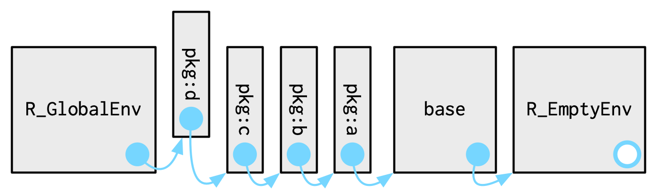
Note that when you attach another package with library(), the parent environment of the global environment changes:
7.4.2 The function environment
A function binds the current environment when it is created. This is called the function environment, and is used for lexical scoping. Across computer languages, functions that capture (or enclose) their environments are called closures, which is why this term is often used interchangeably with function in R’s documentation.
You can get the function environment with fn_env():
y <- 1
f <- function(x) x + y
fn_env(f)
#> <environment: R_GlobalEnv>
Use environment(f) to access the environment of function f.
In diagrams, I’ll draw a function as a rectangle with a rounded end that binds an environment.
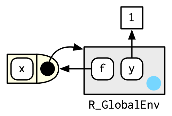
In this case, f() binds the environment that binds the name f to the function. But that’s not always the case: in the following example g is bound in a new environment e, but g() binds the global environment. The distinction between binding and being bound by is subtle but important; the difference is how we find g versus how g finds its variables.
e <- env()
e$g <- function() 1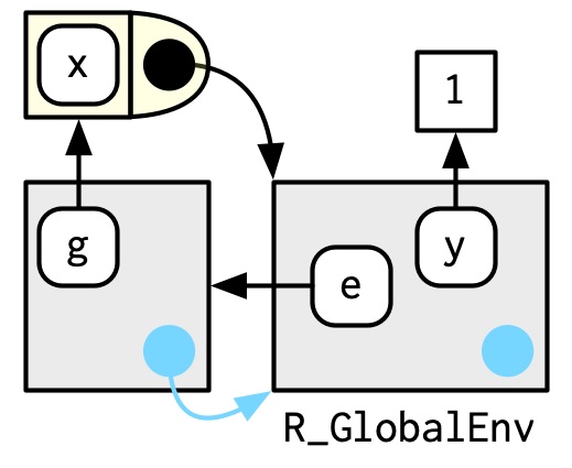
7.4.3 Namespaces
In the diagram above, you saw that the parent environment of a package varies based on what other packages have been loaded. This seems worrying: doesn’t that mean that the package will find different functions if packages are loaded in a different order? The goal of namespaces is to make sure that this does not happen, and that every package works the same way regardless of what packages are attached by the user.
For example, take sd():
sd
#> function (x, na.rm = FALSE)
#> sqrt(var(if (is.vector(x) || is.factor(x)) x else as.double(x),
#> na.rm = na.rm))
#> <bytecode: 0x5556a5eb3690>
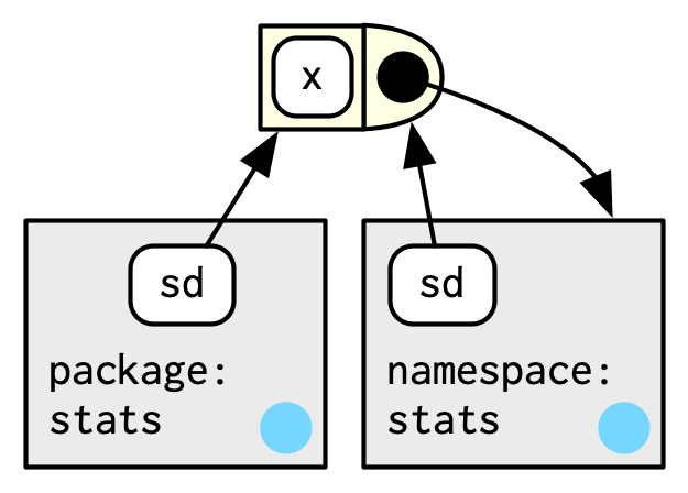
#> <environment: namespace:stats>sd() is defined in terms of var(), so you might worry that the result of sd() would be affected by any function called var() either in the global environment, or in one of the other attached packages. R avoids this problem by taking advantage of the function versus binding environment described above. Every function in a package is associated with a pair of environments: the package environment, which you learned about earlier, and the namespace environment.
The package environment is the external interface to the package. It’s how you, the R user, find a function in an attached package or with
::. Its parent is determined by search path, i.e. the order in which packages have been attached.The namespace environment is the internal interface to the package. The package environment controls how we find the function; the namespace controls how the function finds its variables.
Every binding in the package environment is also found in the namespace environment; this ensures every function can use every other function in the package. But some bindings only occur in the namespace environment. These are known as internal or non-exported objects, which make it possible to hide internal implementation details from the user.
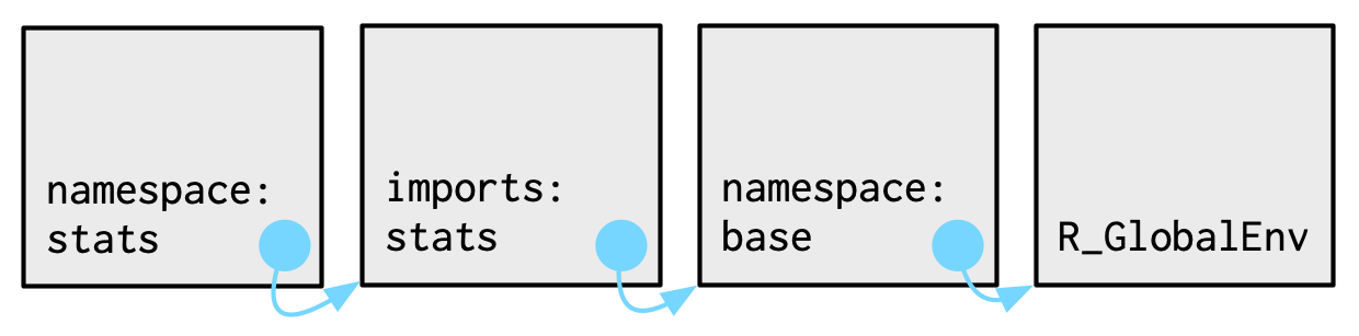
Every namespace environment has the same set of ancestors:
Each namespace has an imports environment that contains bindings to all the functions used by the package. The imports environment is controlled by the package developer with the
NAMESPACEfile.Explicitly importing every base function would be tiresome, so the parent of the imports environment is the base namespace. The base namespace contains the same bindings as the base environment, but it has a different parent.
The parent of the base namespace is the global environment. This means that if a binding isn’t defined in the imports environment the package will look for it in the usual way. This is usually a bad idea (because it makes code depend on other loaded packages), so
R CMD checkautomatically warns about such code. It is needed primarily for historical reasons, particularly due to how S3 method dispatch works.
Putting all these diagrams together we get:
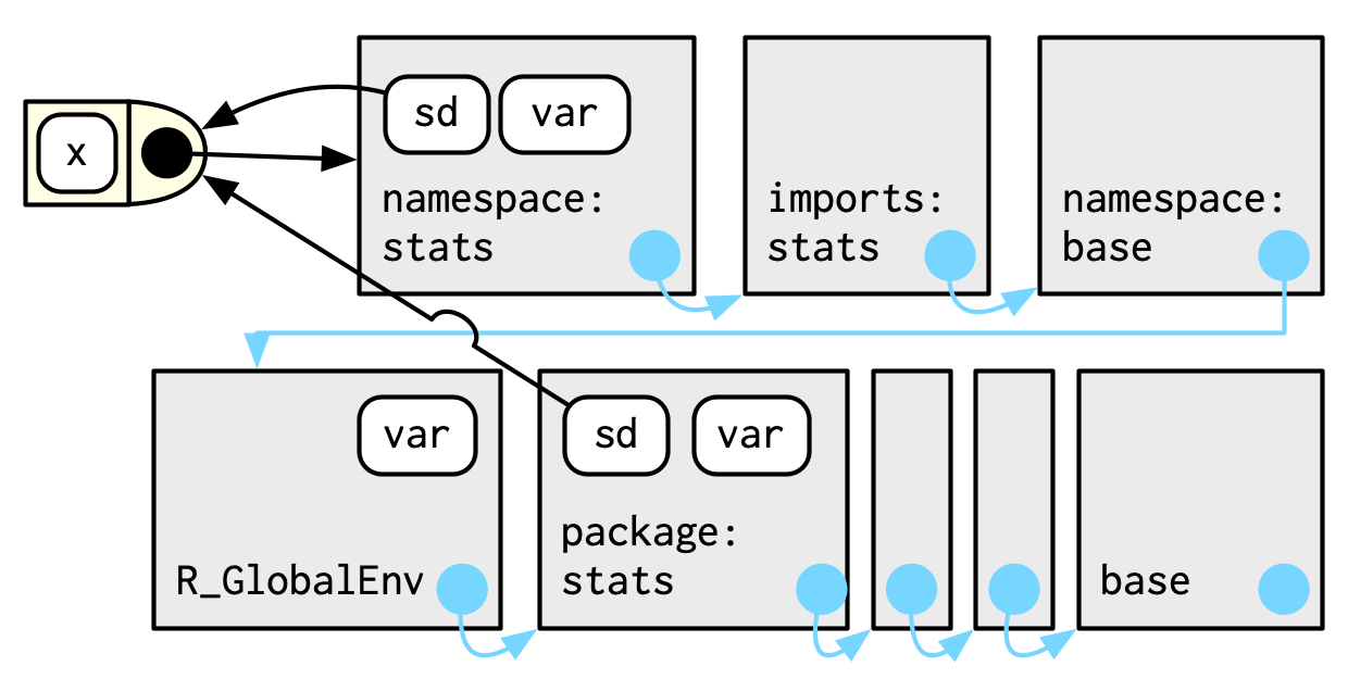
So when sd() looks for the value of var it always finds it in a sequence of environments determined by the package developer, but not by the package user. This ensures that package code always works the same way regardless of what packages have been attached by the user.
There’s no direct link between the package and namespace environments; the link is defined by the function environments.
7.4.4 Execution environments
The last important topic we need to cover is the execution environment. What will the following function return the first time it’s run? What about the second?
g <- function(x) {
  if (!env_has(current_env(), "a")) {
    message("Defining a")
    a <- 1
  } else {
    a <- a + 1
  }
  a
}
Think about it for a moment before you read on.
g(10)
#> Defining a
#> [1] 1
g(10)
#> Defining a
#> [1] 1
This function returns the same value every time because of the fresh start principle, described in Section 6.4.3. Each time a function is called, a new environment is created to host execution. This is called the execution environment, and its parent is the function environment. Let’s illustrate that process with a simpler function. Figure 7.1 illustrates the graphical conventions: I draw execution environments with an indirect parent; the parent environment is found via the function environment.
h <- function(x) {
  # 1.
  a <- 2 # 2.
  x + a
}
y <- h(1) # 3.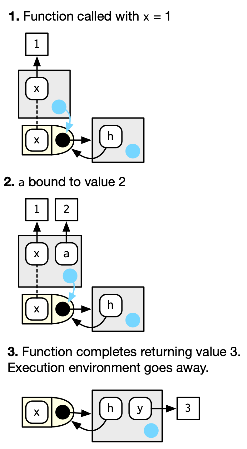
Figure 7.1: The execution environment of a simple function call. Note that the parent of the execution environment is the function environment.
An execution environment is usually ephemeral; once the function has completed, the environment will be garbage collected. There are several ways to make it stay around for longer. The first is to explicitly return it:
h2 <- function(x) {
  a <- x * 2
  current_env()
}

e <- h2(x = 10)
env_print(e)
#> <environment: 0x5556aa59c640>
#> parent: <environment: global>
#> bindings:
#>  * a: <dbl>
#>  * x: <dbl>
fn_env(h2)
#> <environment: R_GlobalEnv>
Another way to capture it is to return an object with a binding to that environment, like a function. The following example illustrates that idea with a function factory, plus(). We use that factory to create a function called plus_one().
There’s a lot going on in the diagram because the enclosing environment of plus_one() is the execution environment of plus().
plus <- function(x) {
  function(y) x + y
}

plus_one <- plus(1)
plus_one
#> function(y) x + y
#> <environment: 0x5556a951de38>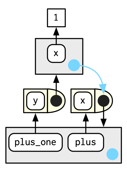
What happens when we call plus_one()? Its execution environment will have the captured execution environment of plus() as its parent:
plus_one(2)
#> [1] 3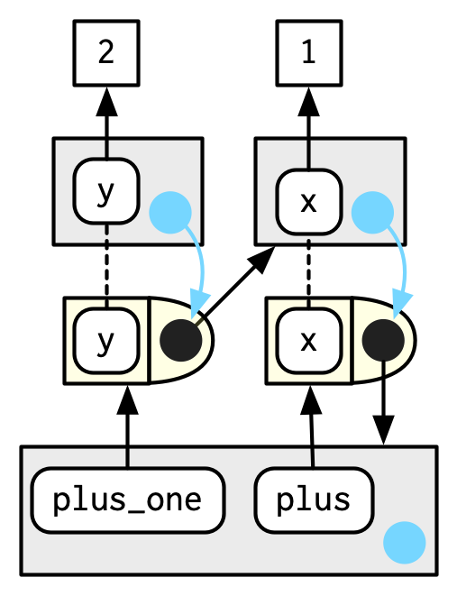
You’ll learn more about function factories in Section 10.2.
7.4.5 Exercises
How is
search_envs()different fromenv_parents(global_env())?Draw a diagram that shows the enclosing environments of this function:
f1 <- function(x1) {
  f2 <- function(x2) {
    f3 <- function(x3) {
      x1 + x2 + x3
    }
    f3(3)
  }
  f2(2)
}
f1(1)
Write an enhanced version of
str()that provides more information about functions. Show where the function was found and what environment it was defined in.
Note the difference between attached and loaded. A package is loaded automatically if you access one of its functions using
::; it is only attached to the search path bylibrary()orrequire().↩︎