10.4 Statistical factories
More motivating examples for function factories come from statistics:
- The Box-Cox transformation.
- Bootstrap resampling.
- Maximum likelihood estimation.
All of these examples can be tackled without function factories, but I think function factories are a good fit for these problems and provide elegant solutions. These examples expect some statistical background, so feel free to skip if they don’t make much sense to you.
10.4.1 Box-Cox transformation
The Box-Cox transformation (a type of power transformation) is a flexible transformation often used to transform data towards normality. It has a single parameter, \(\lambda\), which controls the strength of the transformation. We could express the transformation as a simple two argument function:
boxcox1 <- function(x, lambda) {
  stopifnot(length(lambda) == 1)

  if (lambda == 0) {
    log(x)
  } else {
    (x ^ lambda - 1) / lambda
  }
}
But re-formulating as a function factory makes it easy to explore its behaviour with stat_function():
boxcox2 <- function(lambda) {
if (lambda == 0) {
function(x) log(x)
} else {
function(x) (x ^ lambda - 1) / lambda
}
}
stat_boxcox <- function(lambda) {
stat_function(aes(colour = lambda), fun = boxcox2(lambda), size = 1)
}
ggplot(data.frame(x = c(0, 5)), aes(x)) +
lapply(c(0.5, 1, 1.5), stat_boxcox) +
scale_colour_viridis_c(limits = c(0, 1.5))
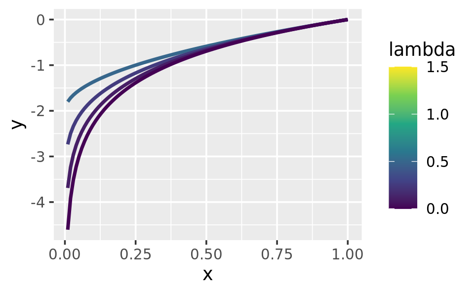
# visually, log() does seem to make sense as the transformation
# for lambda = 0; as values get smaller and smaller, the function
# gets close and closer to a log transformation
ggplot(data.frame(x = c(0.01, 1)), aes(x)) +
lapply(c(0.5, 0.25, 0.1, 0), stat_boxcox) +
scale_colour_viridis_c(limits = c(0, 1.5))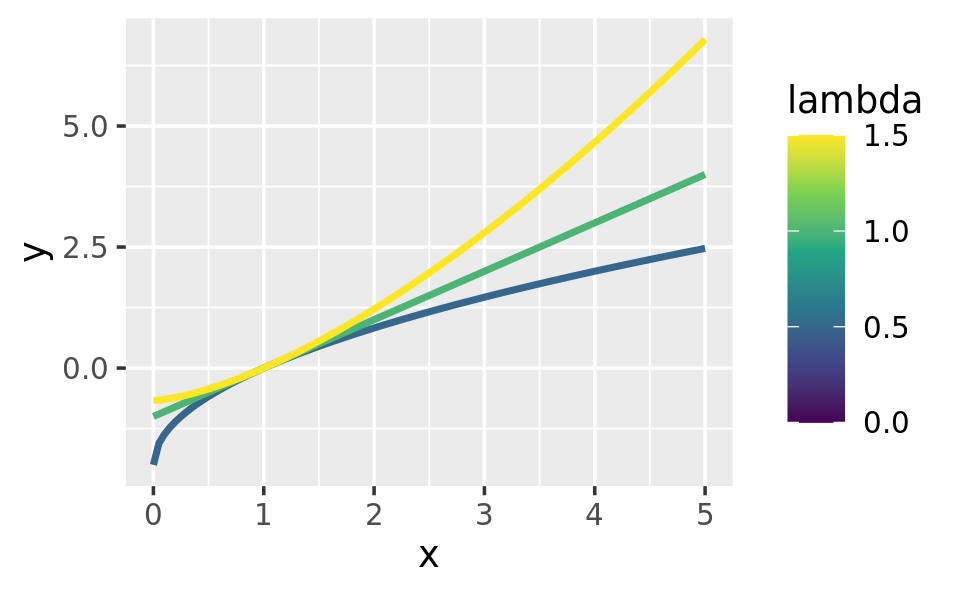
In general, this allows you to use a Box-Cox transformation with any function that accepts a unary transformation function: you don’t have to worry about that function providing ... to pass along additional arguments. I also think that the partitioning of lambda and x into two different function arguments is natural since lambda plays quite a different role than x.
10.4.2 Bootstrap generators
Function factories are a useful approach for bootstrapping. Instead of thinking about a single bootstrap (you always need more than one!), you can think about a bootstrap generator, a function that yields a fresh bootstrap every time it is called:
boot_permute <- function(df, var) {
  n <- nrow(df)
  force(var)

  function() {
    col <- df[[var]]
    col[sample(n, replace = TRUE)]
  }
}

boot_mtcars1 <- boot_permute(mtcars, "mpg")
head(boot_mtcars1())
#> [1] 16.4 22.8 22.8 22.8 16.4 19.2
head(boot_mtcars1())
#> [1] 17.8 18.7 30.4 30.4 16.4 21.0
The advantage of a function factory is more clear with a parametric bootstrap where we have to first fit a model. We can do this setup step once, when the factory is called, rather than once every time we generate the bootstrap:
boot_model <- function(df, formula) {
  mod <- lm(formula, data = df)
  fitted <- unname(fitted(mod))
  resid <- unname(resid(mod))
  rm(mod)

  function() {
    fitted + sample(resid)
  }
}

boot_mtcars2 <- boot_model(mtcars, mpg ~ wt)
head(boot_mtcars2())
#> [1] 25.0 24.0 21.7 19.2 24.9 16.0
head(boot_mtcars2())
#> [1] 27.4 21.0 20.3 19.4 16.3 21.3
I use rm(mod) because linear model objects are quite large (they include complete copies of the model matrix and input data) and I want to keep the manufactured function as small as possible.
10.4.3 Maximum likelihood estimation
The goal of maximum likelihood estimation (MLE) is to find the parameter values for a distribution that make the observed data most likely. To do MLE, you start with a probability function. For example, take the Poisson distribution. If we know \(\lambda\), we can compute the probability of getting a vector \(\mathbf{x}\) of values (\(x_1\), \(x_2\), …, \(x_n\)) by multiplying the Poisson probability function as follows:
\[ P(\lambda, \mathbf{x}) = \prod_{i=1}^{n} \frac{\lambda ^ {x_i} e^{-\lambda}}{x_i!} \]
In statistics, we almost always work with the log of this function. The log is a monotonic transformation which preserves important properties (i.e. the extrema occur in the same place), but has specific advantages:
The log turns a product into a sum, which is easier to work with.
Multiplying small numbers yields even smaller numbers, which makes the floating point approximation used by a computer less accurate.
Let’s apply a log transformation to this probability function and simplify it as much as possible:
\[ \log(P(\lambda, \mathbf{x})) = \sum_{i=1}^{n} \log(\frac{\lambda ^ {x_i} e^{-\lambda}}{x_i!}) \]
\[ \log(P(\lambda, \mathbf{x})) = \sum_{i=1}^{n} \left( x_i \log(\lambda) - \lambda - \log(x_i!) \right) \]
\[ \log(P(\lambda, \mathbf{x})) = \sum_{i=1}^{n} x_i \log(\lambda) - \sum_{i=1}^{n} \lambda - \sum_{i=1}^{n} \log(x_i!) \]
\[ \log(P(\lambda, \mathbf{x})) = \log(\lambda) \sum_{i=1}^{n} x_i - n \lambda - \sum_{i=1}^{n} \log(x_i!) \]
We can now turn this function into an R function. The R function is quite elegant because R is vectorised and, because it’s a statistical programming language, R comes with built-in functions like the log-factorial (lfactorial()).
lprob_poisson <- function(lambda, x) {
  n <- length(x)
  (log(lambda) * sum(x)) - (n * lambda) - sum(lfactorial(x))
}
Consider this vector of observations:
x1 <- c(41, 30, 31, 38, 29, 24, 30, 29, 31, 38)We can use lprob_poisson() to compute the (logged) probability of x1 for different values of lambda.
lprob_poisson(10, x1)
#> [1] -184
lprob_poisson(20, x1)
#> [1] -61.1
lprob_poisson(30, x1)
#> [1] -31
So far we’ve been thinking of lambda as fixed and known and the function told us the probability of getting different values of x. But in real-life, we observe x and it is lambda that is unknown. The likelihood is the probability function seen through this lens: we want to find the lambda that makes the observed x the most likely. That is, given x, what value of lambda gives us the highest value of lprob_poisson()?
In statistics, we highlight this change in perspective by writing \(f_{\mathbf{x}}(\lambda)\) instead of \(f(\lambda, \mathbf{x})\). In R, we can use a function factory. We provide x and generate a function with a single parameter, lambda:
ll_poisson1 <- function(x) {
  n <- length(x)

  function(lambda) {
    log(lambda) * sum(x) - n * lambda - sum(lfactorial(x))
  }
}
(We don’t need force() because length() implicitly forces evaluation of x.)
One nice thing about this approach is that we can do some precomputation: any term that only involves x can be computed once in the factory. This is useful because we’re going to need to call this function many times to find the best lambda.
ll_poisson2 <- function(x) {
  n <- length(x)
  sum_x <- sum(x)
  c <- sum(lfactorial(x))

  function(lambda) {
    log(lambda) * sum_x - n * lambda - c
  }
}
Now we can use this function to find the value of lambda that maximizes the (log) likelihood:
ll1 <- ll_poisson2(x1)

ll1(10)
#> [1] -184
ll1(20)
#> [1] -61.1
ll1(30)
#> [1] -31
Rather than trial and error, we can automate the process of finding the best value with optimise(). It will evaluate ll1() many times, using mathematical tricks to narrow in on the largest value as quickly as possible. The results tell us that the highest value is -30.27 which occurs when lambda = 32.1:
optimise(ll1, c(0, 100), maximum = TRUE)
#> $maximum
#> [1] 32.1
#>
#> $objective
#> [1] -30.3
Now, we could have solved this problem without using a function factory because optimise() passes ... on to the function being optimised. That means we could use the log-probability function directly:
optimise(lprob_poisson, c(0, 100), x = x1, maximum = TRUE)
#> $maximum
#> [1] 32.1
#>
#> $objective
#> [1] -30.3
The advantage of using a function factory here is fairly small, but there are two niceties:
We can precompute some values in the factory, saving computation time in each iteration.
The two-level design better reflects the mathematical structure of the underlying problem.
These advantages get bigger in more complex MLE problems, where you have multiple parameters and multiple data vectors.
10.4.4 Exercises
In
boot_model(), why don’t I need to force the evaluation ofdformodel?Why might you formulate the Box-Cox transformation like this?
boxcox3 <- function(x) {
  function(lambda) {
    if (lambda == 0) {
      log(x)
    } else {
      (x ^ lambda - 1) / lambda
    }
  }
}
Why don’t you need to worry that
boot_permute()stores a copy of the data inside the function that it generates?How much time does
ll_poisson2()save compared toll_poisson1()? Usebench::mark()to see how much faster the optimisation occurs. How does changing the length ofxchange the results?