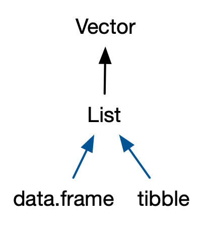
3.6 Data frames and tibbles
The two most important S3 vectors built on top of lists are data frames and tibbles.
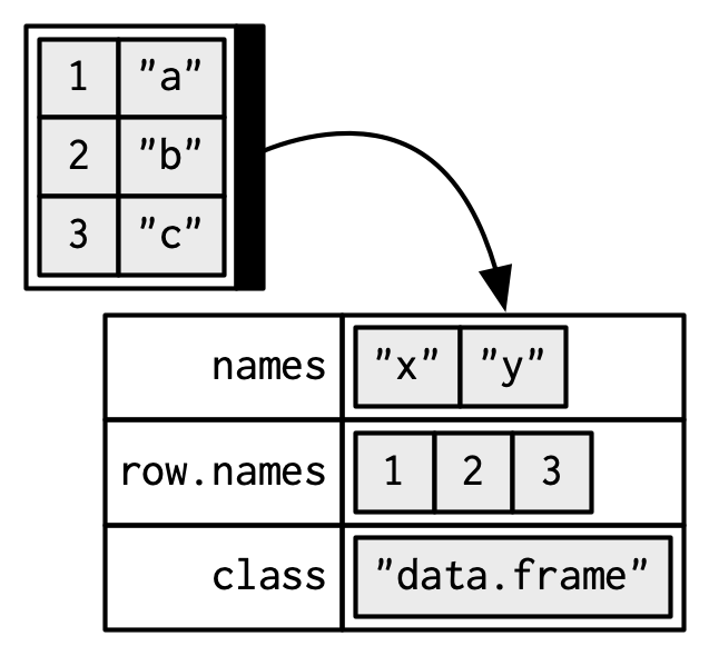
If you do data analysis in R, you’re going to be using data frames. A data frame is a named list of vectors with attributes for (column) names, row.names20, and its class, “data.frame”:
df1 <- data.frame(x = 1:3, y = letters[1:3])
typeof(df1)
#> [1] "list"

attributes(df1)
#> $names
#> [1] "x" "y"
#>
#> $class
#> [1] "data.frame"
#>
#> $row.names
#> [1] 1 2 3
In contrast to a regular list, a data frame has an additional constraint: the length of each of its vectors must be the same. This gives data frames their rectangular structure and explains why they share the properties of both matrices and lists:
A data frame has
rownames()21 andcolnames(). Thenames()of a data frame are the column names.A data frame has
nrow()rows andncol()columns. Thelength()of a data frame gives the number of columns.
Data frames are one of the biggest and most important ideas in R, and one of the things that make R different from other programming languages. However, in the over 20 years since their creation, the ways that people use R have changed, and some of the design decisions that made sense at the time data frames were created now cause frustration.
This frustration lead to the creation of the tibble (Müller and Wickham 2018), a modern reimagining of the data frame. Tibbles are designed to be (as much as possible) drop-in replacements for data frames that fix those frustrations. A concise, and fun, way to summarise the main differences is that tibbles are lazy and surly: they do less and complain more. You’ll see what that means as you work through this section.
Tibbles are provided by the tibble package and share the same structure as data frames. The only difference is that the class vector is longer, and includes tbl_df. This allows tibbles to behave differently in the key ways which we’ll discuss below.
library(tibble)

df2 <- tibble(x = 1:3, y = letters[1:3])
typeof(df2)
#> [1] "list"

attributes(df2)
#> $names
#> [1] "x" "y"
#>
#> $row.names
#> [1] 1 2 3
#>
#> $class
#> [1] "tbl_df"     "tbl"        "data.frame"
3.6.1 Creating
You create a data frame by supplying name-vector pairs to data.frame():
df <- data.frame(
  x = 1:3,
  y = c("a", "b", "c")
)
str(df)
#> 'data.frame':    3 obs. of  2 variables:
#>  $ x: int  1 2 3
#>  $ y: chr  "a" "b" "c"
Beware of the default conversion of strings to factors. Use stringsAsFactors = FALSE to suppress this and keep character vectors as character vectors:
df1 <- data.frame(
  x = 1:3,
  y = c("a", "b", "c"),
  stringsAsFactors = FALSE
)
str(df1)
#> 'data.frame':    3 obs. of  2 variables:
#>  $ x: int  1 2 3
#>  $ y: chr  "a" "b" "c"
Creating a tibble is similar to creating a data frame. The difference between the two is that tibbles never coerce their input (this is one feature that makes them lazy):
df2 <- tibble(
  x = 1:3,
  y = c("a", "b", "c")
)
str(df2)
#> tibble [3 × 2] (S3: tbl_df/tbl/data.frame)
#>  $ x: int [1:3] 1 2 3
#>  $ y: chr [1:3] "a" "b" "c"
Additionally, while data frames automatically transform non-syntactic names (unless check.names = FALSE), tibbles do not (although they do print non-syntactic names surrounded by `).
names(data.frame(`1` = 1))
#> [1] "X1"

names(tibble(`1` = 1))
#> [1] "1"
While every element of a data frame (or tibble) must have the same length, both data.frame() and tibble() will recycle shorter inputs. However, while data frames automatically recycle columns that are an integer multiple of the longest column, tibbles will only recycle vectors of length one.
data.frame(x = 1:4, y = 1:2)
#>   x y
#> 1 1 1
#> 2 2 2
#> 3 3 1
#> 4 4 2
data.frame(x = 1:4, y = 1:3)
#> Error in data.frame(x = 1:4, y = 1:3): arguments imply differing number of
#> rows: 4, 3

tibble(x = 1:4, y = 1)
#> # A tibble: 4 x 2
#>       x     y
#>   <int> <dbl>
#> 1     1     1
#> 2     2     1
#> 3     3     1
#> 4     4     1
tibble(x = 1:4, y = 1:2)
#> Error: Tibble columns must have compatible sizes.
#> * Size 4: Existing data.
#> * Size 2: Column `y`.
#> ℹ Only values of size one are recycled.
There is one final difference: tibble() allows you to refer to variables created during construction:
tibble(
  x = 1:3,
  y = x * 2
)
#> # A tibble: 3 x 2
#>       x     y
#>   <int> <dbl>
#> 1     1     2
#> 2     2     4
#> 3     3     6
(Inputs are evaluated left-to-right.)
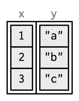
When drawing data frames and tibbles, rather than focussing on the implementation details, i.e. the attributes:
I’ll draw them the same way as a named list, but arrange them to emphasise their columnar structure.
3.6.2 Row names
Data frames allow you to label each row with a name, a character vector containing only unique values:
df3 <- data.frame(
  age = c(35, 27, 18),
  hair = c("blond", "brown", "black"),
  row.names = c("Bob", "Susan", "Sam")
)
df3
#>       age  hair
#> Bob    35 blond
#> Susan  27 brown
#> Sam    18 black
You can get and set row names with rownames(), and you can use them to subset rows:
rownames(df3)
#> [1] "Bob"   "Susan" "Sam"

df3["Bob", ]
#>     age  hair
#> Bob  35 blond
Row names arise naturally if you think of data frames as 2D structures like matrices: columns (variables) have names so rows (observations) should too. Most matrices are numeric, so having a place to store character labels is important. But this analogy to matrices is misleading because matrices possess an important property that data frames do not: they are transposable. In matrices the rows and columns are interchangeable, and transposing a matrix gives you another matrix (transposing again gives you the original matrix). With data frames, however, the rows and columns are not interchangeable: the transpose of a data frame is not a data frame.
There are three reasons why row names are undesirable:
Metadata is data, so storing it in a different way to the rest of the data is fundamentally a bad idea. It also means that you need to learn a new set of tools to work with row names; you can’t use what you already know about manipulating columns.
Row names are a poor abstraction for labelling rows because they only work when a row can be identified by a single string. This fails in many cases, for example when you want to identify a row by a non-character vector (e.g. a time point), or with multiple vectors (e.g. position, encoded by latitude and longitude).
Row names must be unique, so any duplication of rows (e.g. from bootstrapping) will create new row names. If you want to match rows from before and after the transformation, you’ll need to perform complicated string surgery.
df3[c(1, 1, 1), ]
#>       age  hair
#> Bob    35 blond
#> Bob.1  35 blond
#> Bob.2  35 blond
For these reasons, tibbles do not support row names. Instead the tibble package provides tools to easily convert row names into a regular column with either rownames_to_column(), or the rownames argument in as_tibble():
as_tibble(df3, rownames = "name")
#> # A tibble: 3 x 3
#>   name    age hair
#>   <chr> <dbl> <chr>
#> 1 Bob      35 blond
#> 2 Susan    27 brown
#> 3 Sam      18 black
3.6.3 Printing
One of the most obvious differences between tibbles and data frames is how they print. I assume that you’re already familiar with how data frames are printed, so here I’ll highlight some of the biggest differences using an example dataset included in the dplyr package:
dplyr::starwars
#> # A tibble: 87 x 14
#>    name  height  mass hair_color skin_color eye_color birth_year sex   gender
#>    <chr>  <int> <dbl> <chr>      <chr>      <chr>          <dbl> <chr> <chr>
#>  1 Luke…    172    77 blond      fair       blue            19   male  mascu…
#>  2 C-3PO    167    75 <NA>       gold       yellow         112   none  mascu…
#>  3 R2-D2     96    32 <NA>       white, bl… red             33   none  mascu…
#>  4 Dart…    202   136 none       white      yellow          41.9 male  mascu…
#>  5 Leia…    150    49 brown      light      brown           19   fema… femin…
#>  6 Owen…    178   120 brown, gr… light      blue            52   male  mascu…
#>  7 Beru…    165    75 brown      light      blue            47   fema… femin…
#>  8 R5-D4     97    32 <NA>       white, red red             NA   none  mascu…
#>  9 Bigg…    183    84 black      light      brown           24   male  mascu…
#> 10 Obi-…    182    77 auburn, w… fair       blue-gray       57   male  mascu…
#> # … with 77 more rows, and 5 more variables: homeworld <chr>, species <chr>,
#> #   films <list>, vehicles <list>, starships <list>
Tibbles only show the first 10 rows and all the columns that will fit on screen. Additional columns are shown at the bottom.
Each column is labelled with its type, abbreviated to three or four letters.
Wide columns are truncated to avoid having a single long string occupy an entire row. (This is still a work in progress: it’s a tricky tradeoff between showing as many columns as possible and showing columns in their entirety.)
When used in console environments that support it, colour is used judiciously to highlight important information, and de-emphasise supplemental details.
3.6.4 Subsetting
As you will learn in Chapter 4, you can subset a data frame or a tibble like a 1D structure (where it behaves like a list), or a 2D structure (where it behaves like a matrix).
In my opinion, data frames have two undesirable subsetting behaviours:
When you subset columns with
df[, vars], you will get a vector ifvarsselects one variable, otherwise you’ll get a data frame. This is a frequent source of bugs when using[in a function, unless you always remember to usedf[, vars, drop = FALSE].When you attempt to extract a single column with
df$xand there is no columnx, a data frame will instead select any variable that starts withx. If no variable starts withx,df$xwill returnNULL. This makes it easy to select the wrong variable or to select a variable that doesn’t exist.
Tibbles tweak these behaviours so that a [ always returns a tibble, and a $ doesn’t do partial matching and warns if it can’t find a variable (this is what makes tibbles surly).
df1 <- data.frame(xyz = "a")
df2 <- tibble(xyz = "a")

str(df1$x)
#>  chr "a"
str(df2$x)
#> Warning: Unknown or uninitialised column: `x`.
#>  NULL
A tibble’s insistence on returning a data frame from [ can cause problems with legacy code, which often uses df[, "col"] to extract a single column. If you want a single column, I recommend using df[["col"]]. This clearly communicates your intent, and works with both data frames and tibbles.
3.6.5 Testing and coercing
To check if an object is a data frame or tibble, use is.data.frame():
is.data.frame(df1)
#> [1] TRUE
is.data.frame(df2)
#> [1] TRUE
Typically, it should not matter if you have a tibble or data frame, but if you need to be certain, use is_tibble():
is_tibble(df1)
#> [1] FALSE
is_tibble(df2)
#> [1] TRUE
You can coerce an object to a data frame with as.data.frame() or to a tibble with as_tibble().
3.6.6 List columns
Since a data frame is a list of vectors, it is possible for a data frame to have a column that is a list. This is very useful because a list can contain any other object: this means you can put any object in a data frame. This allows you to keep related objects together in a row, no matter how complex the individual objects are. You can see an application of this in the “Many Models” chapter of R for Data Science, http://r4ds.had.co.nz/many-models.html.
List-columns are allowed in data frames but you have to do a little extra work by either adding the list-column after creation or wrapping the list in I()22.
df <- data.frame(x = 1:3)
df$y <- list(1:2, 1:3, 1:4)

data.frame(
  x = 1:3,
  y = I(list(1:2, 1:3, 1:4))
)
#>   x          y
#> 1 1       1, 2
#> 2 2    1, 2, 3
#> 3 3 1, 2, 3, 4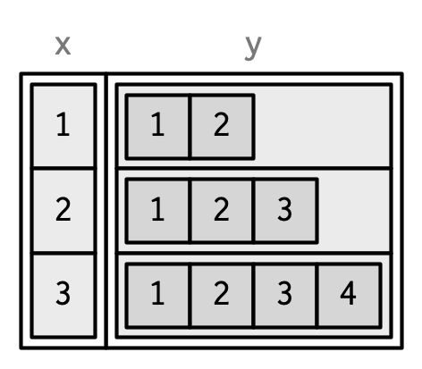
List columns are easier to use with tibbles because they can be directly included inside tibble() and they will be printed tidily:
tibble(
  x = 1:3,
  y = list(1:2, 1:3, 1:4)
)
#> # A tibble: 3 x 2
#>       x y
#>   <int> <list>
#> 1     1 <int [2]>
#> 2     2 <int [3]>
#> 3     3 <int [4]>
3.6.7 Matrix and data frame columns
As long as the number of rows matches the data frame, it’s also possible to have a matrix or array as a column of a data frame. (This requires a slight extension to our definition of a data frame: it’s not the length() of each column that must be equal, but the NROW().) As for list-columns, you must either add it after creation, or wrap it in I().
dfm <- data.frame(
  x = 1:3 * 10
)
dfm$y <- matrix(1:9, nrow = 3)
dfm$z <- data.frame(a = 3:1, b = letters[1:3], stringsAsFactors = FALSE)

str(dfm)
#> 'data.frame':    3 obs. of  3 variables:
#>  $ x: num  10 20 30
#>  $ y: int [1:3, 1:3] 1 2 3 4 5 6 7 8 9
#>  $ z:'data.frame':   3 obs. of  2 variables:
#>   ..$ a: int  3 2 1
#>   ..$ b: chr  "a" "b" "c"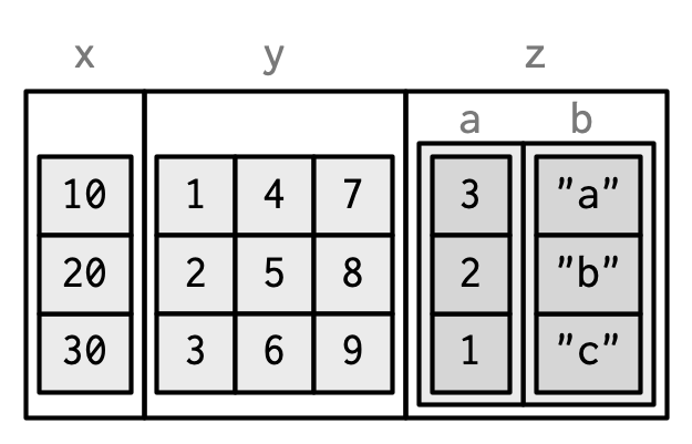
Matrix and data frame columns require a little caution. Many functions that work with data frames assume that all columns are vectors. Also, the printed display can be confusing.
dfm[1, ]
#>    x y.1 y.2 y.3 z.a z.b
#> 1 10   1   4   7   3   a
3.6.8 Exercises
Can you have a data frame with zero rows? What about zero columns?
What happens if you attempt to set rownames that are not unique?
If
dfis a data frame, what can you say aboutt(df), andt(t(df))? Perform some experiments, making sure to try different column types.What does
as.matrix()do when applied to a data frame with columns of different types? How does it differ fromdata.matrix()?
References
Müller, Kirill, and Hadley Wickham. 2018. Tibble: Simple Data Frames. http://tibble.tidyverse.org/.
Row names are one of the most surprisingly complex data structures in R. They’ve also been a persistent source of performance issues over the years. The most straightforward implementation is a character or integer vector, with one element for each row. But there’s also a compact representation for “automatic” row names (consecutive integers), created by
.set_row_names(). R 3.5 has a special way of deferring integer to character conversion that is specifically designed to speed uplm(); see https://svn.r-project.org/R/branches/ALTREP/ALTREP.html#deferred_string_conversions for details.↩︎Technically, you are encouraged to use
row.names(), notrownames()with data frames, but this distinction is rarely important.↩︎I()is short for identity and is often used to indicate that an input should be left as is, and not automatically transformed.↩︎