13.4 Aesthetic mappings
The aesthetic mappings, defined with aes(), describe how variables are mapped to visual properties or aesthetics. aes() takes a sequence of aesthetic-variable pairs like this:
aes(x = displ, y = hwy, colour = class)(If you’re American, you can use color, and behind the scenes ggplot2 will correct your spelling ;)
Here we map x-position to displ, y-position to hwy, and colour to class. The names for the first two arguments can be omitted, in which case they correspond to the x and y variables. That makes this specification equivalent to the one above:
aes(displ, hwy, colour = class)While you can do data manipulation in aes(), e.g. aes(log(carat), log(price)), it’s best to only do simple calculations. It’s better to move complex transformations out of the aes() call and into an explicit dplyr::mutate() call. This makes it easier to check your work and it’s often faster because you need only do the transformation once, not every time the plot is drawn.
Never refer to a variable with $ (e.g., diamonds$carat) in aes(). This breaks containment, so that the plot no longer contains everything it needs, and causes problems if ggplot2 changes the order of the rows, as it does when faceting.
13.4.1 Specifying the aesthetics in the plot vs. in the layers
Aesthetic mappings can be supplied in the initial ggplot() call, in individual layers, or in some combination of both. All of these calls create the same plot specification:
ggplot(mpg, aes(displ, hwy, colour = class)) +
  geom_point()
ggplot(mpg, aes(displ, hwy)) +
  geom_point(aes(colour = class))
ggplot(mpg, aes(displ)) +
  geom_point(aes(y = hwy, colour = class))
ggplot(mpg) +
  geom_point(aes(displ, hwy, colour = class))
Within each layer, you can add, override, or remove mappings. For example, if you have a plot using the mpg data that has aes(displ, hwy) as the starting point, the table below illustrates all three operations:
| Operation | Layer aesthetics | Result |
|---|---|---|
| Add | aes(colour = cyl) |
aes(displ, hwy, colour = cyl) |
| Override | aes(y = cty) |
aes(displ, cty) |
| Remove | aes(y = NULL) |
aes(displ) |
If you only have one layer in the plot, the way you specify aesthetics doesn’t make any difference. However, the distinction is important when you start adding additional layers. These two plots are both valid and interesting, but focus on quite different aspects of the data:
ggplot(mpg, aes(displ, hwy, colour = class)) +
geom_point() +
geom_smooth(method = "lm", se = FALSE) +
theme(legend.position = "none")
#> `geom_smooth()` using formula 'y ~ x'
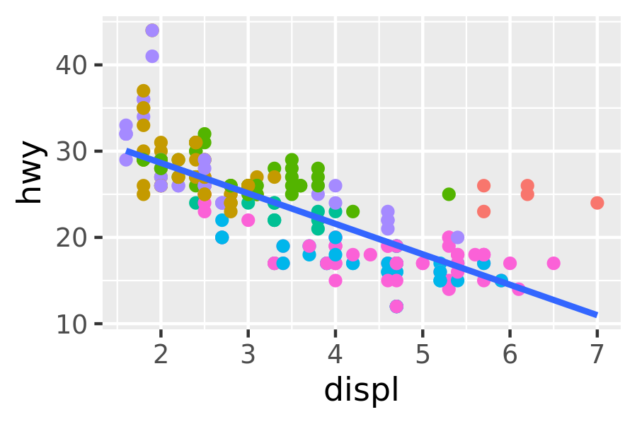
ggplot(mpg, aes(displ, hwy)) +
geom_point(aes(colour = class)) +
geom_smooth(method = "lm", se = FALSE) +
theme(legend.position = "none")
#> `geom_smooth()` using formula 'y ~ x'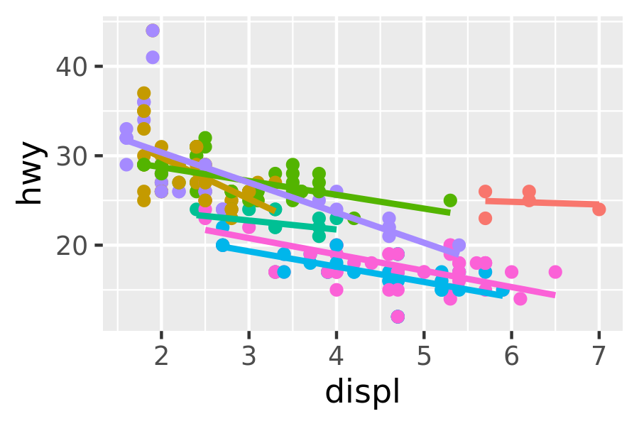
Generally, you want to set up the mappings to illuminate the structure underlying the graphic and minimise typing. It may take some time before the best approach is immediately obvious, so if you’ve iterated your way to a complex graphic, it may be worthwhile to rewrite it to make the structure more clear.
13.4.2 Setting vs. mapping
Instead of mapping an aesthetic property to a variable, you can set it to a single value by specifying it in the layer parameters. We map an aesthetic to a variable (e.g., aes(colour = cut)) or set it to a constant (e.g., colour = "red"). If you want appearance to be governed by a variable, put the specification inside aes(); if you want override the default size or colour, put the value outside of aes().
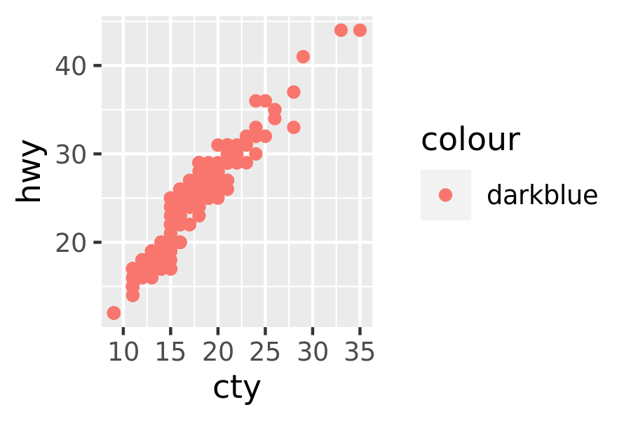
The following plots are created with similar code, but have rather different outputs. The second plot maps (not sets) the colour to the value ‘darkblue’. This effectively creates a new variable containing only the value ‘darkblue’ and then scales it with a colour scale. Because this value is discrete, the default colour scale uses evenly spaced colours on the colour wheel, and since there is only one value this colour is pinkish.
ggplot(mpg, aes(cty, hwy)) +
  geom_point(colour = "darkblue")

ggplot(mpg, aes(cty, hwy)) +
  geom_point(aes(colour = "darkblue"))
A third approach is to map the value, but override the default scale:
ggplot(mpg, aes(cty, hwy)) +
  geom_point(aes(colour = "darkblue")) +
  scale_colour_identity()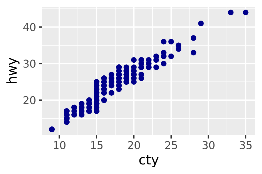
This is most useful if you always have a column that already contains colours. You’ll learn more about that in Section ??.
It’s sometimes useful to map aesthetics to constants. For example, if you want to display multiple layers with varying parameters, you can “name” each layer:
ggplot(mpg, aes(displ, hwy)) +
  geom_point() +
  geom_smooth(aes(colour = "loess"), method = "loess", se = FALSE) +
  geom_smooth(aes(colour = "lm"), method = "lm", se = FALSE) +
  labs(colour = "Method")
#> `geom_smooth()` using formula 'y ~ x'
#> `geom_smooth()` using formula 'y ~ x'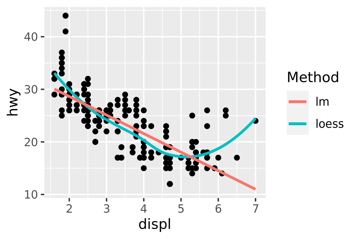
13.4.3 Exercises
Simplify the following plot specifications:
ggplot(mpg) +
  geom_point(aes(mpg$displ, mpg$hwy))

ggplot() +
 geom_point(mapping = aes(y = hwy, x = cty), data = mpg) +
 geom_smooth(data = mpg, mapping = aes(cty, hwy))

ggplot(diamonds, aes(carat, price)) +
  geom_point(aes(log(brainwt), log(bodywt)), data = msleep)
What does the following code do? Does it work? Does it make sense? Why/why not?
ggplot(mpg) +
  geom_point(aes(class, cty)) +
  geom_boxplot(aes(trans, hwy))
What happens if you try to use a continuous variable on the x axis in one layer, and a categorical variable in another layer? What happens if you do it in the opposite order?