21.2 Part 1: A stat
When developing a new layer, you have a choice between developing a Stat or a Geom.
Surprisingly, the decision not guided by whether you want to end up with geom_spring() or stat_spring() because plenty of Stat extensions are used via a geom_*() constructor.
Instead, you need to consider what you’re doing: if you’re just drawing transformed data with pre-existing geom, then you can use a Stat.
Stats are much easier to extend than Geoms as they are simply data-transformation pipelines.
Here we’re drawing a path but circling around instead of going in straight line.
This is good fit of Stat, because we can transform data and then use the existing GeomPath.
21.2.1 Building functionality
When developing a new Stat it’s a good idea to first write the data transformation function.
Here we need a function that takes a start and end point, a diameter, and a tension.
We will define tension to mean “times of diameter moved per revolution minus one”, thus 0 will mean that it doesn’t move at all, and will be forbidden as it would not allow our spring to extend between two points.
We’ll also use a parameter n to give the number of points used per revolution, defining the visual fidelity of the spring.
create_spring <- function(x, y, xend, yend, diameter = 1, tension = 0.75, n = 50) {
  if (tension <= 0) {
    rlang::abort("`tension` must be larger than zero.")
  }
  if (diameter == 0) {
    rlang::abort("`diameter` can not be zero.")
  }
  if (n == 0) {
    rlang::abort("`n` must be greater than zero.")
  }
  # Calculate direct length of segment
  length <- sqrt((x - xend)^2 + (y - yend)^2)

  # Figure out how many revolutions and points we need
  n_revolutions <- length / (diameter * tension)
  n_points <- n * n_revolutions

  # Calculate sequence of radians and x and y offset
  radians <- seq(0, n_revolutions * 2 * pi, length.out = n_points)
  x <- seq(x, xend, length.out = n_points)
  y <- seq(y, yend, length.out = n_points)

  # Create the new data
  data.frame(
    x = cos(radians) * diameter/2 + x,
    y = sin(radians) * diameter/2 + y
  )
}
One nice thing about writing this function is that we can immediately test it out to convince ourselves that the logic works:
spring <- create_spring(
  x = 4, y = 2, xend = 10, yend = 6,
  diameter = 2, tension = 0.75, n = 50
)

ggplot(spring) +
  geom_path(aes(x = x, y = y))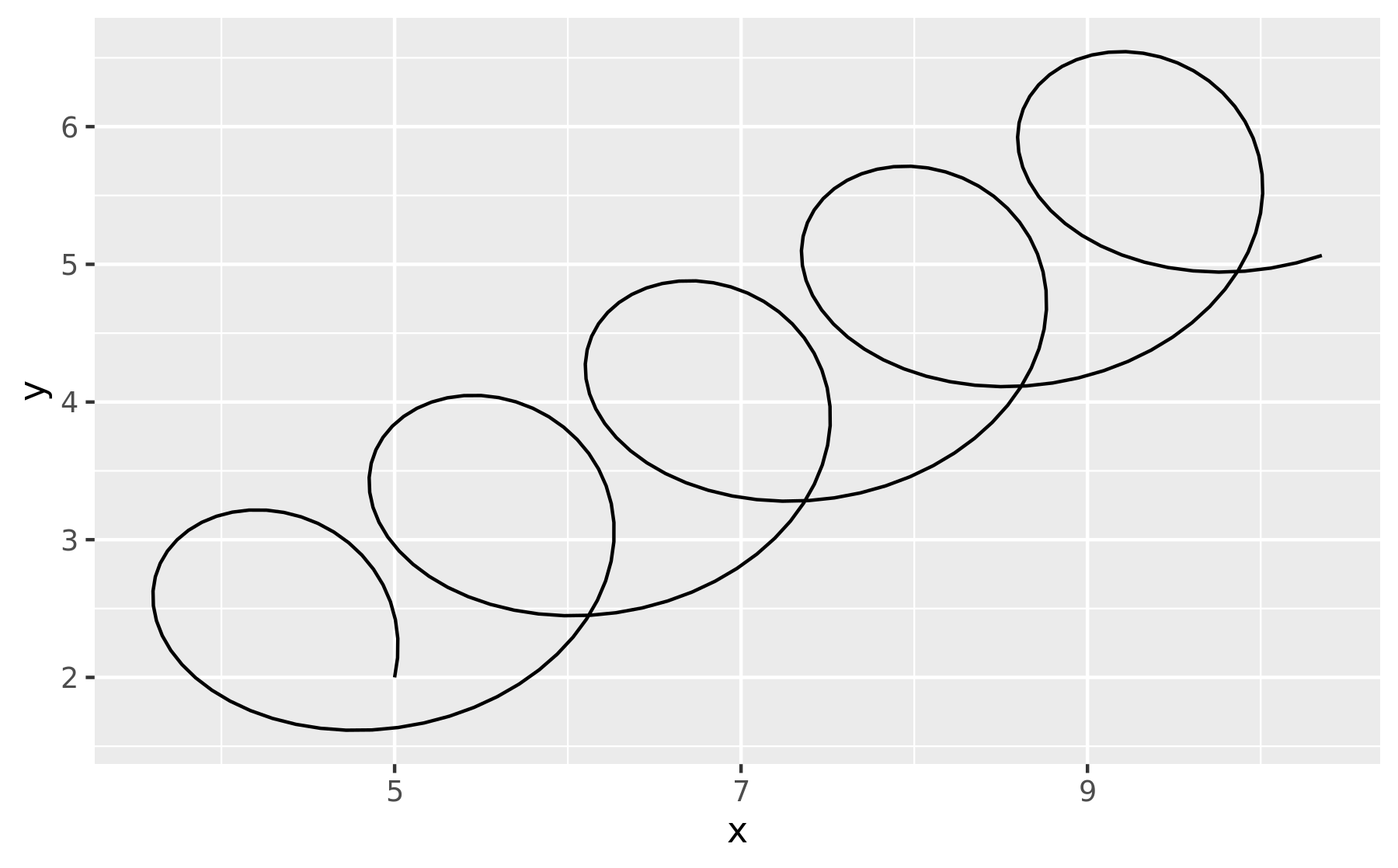
(This would also be a great function to formally test with a unit testing package like testthat)
Now we have the transformation function we can encapsulate it in a new Stat.
We’ll define the Stat below and then work our way through each of the pieces.
`%||%` <- function(x, y) {
  if (is.null(x)) y else x
}

StatSpring <- ggproto("StatSpring", Stat,
  setup_data = function(data, params) {
    if (anyDuplicated(data$group)) {
      data$group <- paste(data$group, seq_len(nrow(data)), sep = "-")
    }
    data
  },
  compute_panel = function(data, scales,
                           diameter = 1,
                           tension = 0.75,
                           n = 50) {
    cols_to_keep <- setdiff(names(data), c("x", "y", "xend", "yend"))
    springs <- lapply(seq_len(nrow(data)), function(i) {
      spring_path <- create_spring(
        data$x[i], data$y[i],
        data$xend[i], data$yend[i],
        diameter = diameter,
        tension = tension,
        n = n
      )
      cbind(spring_path, unclass(data[i, cols_to_keep]))
    })
    do.call(rbind, springs)
  },
  required_aes = c("x", "y", "xend", "yend")
)
We first start with the class definition:
StatSpring <- ggproto("StatSpring", Stat,
  ...
}
This creates a new Stat48 subclass, named StatSpring. ggproto classes always use CamelCase for naming, and the new class is always saved into a variable with the same name.
21.2.2 Methods
Inside the class definition we implement methods by assigning functions to a name.
You can see a complete list of methods by printing the class.
The only methods that you shouldn’t touch are aesthetics and parameters; these are for internal use only.
(To understand exactly what is passed to these methods I highly recommend adding a browser() statement)
print(Stat)
#> <ggproto object: Class Stat, gg>
#>     aesthetics: function
#>     compute_group: function
#>     compute_layer: function
#>     compute_panel: function
#>     default_aes: uneval
#>     extra_params: na.rm
#>     finish_layer: function
#>     non_missing_aes:
#>     optional_aes:
#>     parameters: function
#>     required_aes:
#>     retransform: TRUE
#>     setup_data: function
#>     setup_params: function
As discussed in the last chapter, the most important are the three compute_* methods.
One of these must always be defined (and usually it’s the group or panel version).
Here we use the compute_panel() method because it receives all the data for a single panel.
As a rule of thumb, if the stat operates on multiple rows, start by implementing a compute_group() method, and if the stat operates on single rows, implement a compute_panel() method.
Inside our compute_panel() method we do a bit more than simply call our create_spring() function.
StatSpring$compute_panel
#> <ggproto method>
#>   <Wrapper function>
#>     function (...)
#> f(...)
#>
#>   <Inner function (f)>
#>     function(data, scales,
#>                            diameter = 1,
#>                            tension = 0.75,
#>                            n = 50) {
#>     cols_to_keep <- setdiff(names(data), c("x", "y", "xend", "yend"))
#>     springs <- lapply(seq_len(nrow(data)), function(i) {
#>       spring_path <- create_spring(
#>         data$x[i], data$y[i],
#>         data$xend[i], data$yend[i],
#>         diameter = diameter,
#>         tension = tension,
#>         n = n
#>       )
#>       cbind(spring_path, unclass(data[i, cols_to_keep]))
#>     })
#>     do.call(rbind, springs)
#>   }
We loop over each row of the data and create the points required to draw the spring. Then we combine our new data with all the non-position columns of the row. This is very important, since otherwise the aesthetic mappings to e.g. color and size would be lost. In the end we combine the individual springs into a single data frame that gets returned.
Two other common methods are setup_data and setup_params which allows the class to do early checks and modifications of the parameters and data.
Here our setup_data() method ensures that each input row has a unique group aesthetic.
This is important because the we’re going to draw our springs with GeomPath(), so we need to make sure that each row has it’s own id so the springs don’t get tangled.
The group aesthetic is sometimes used to carry metadata so we preserve the existing value, and pasting on a unique id if needed.
StatSpring$setup_data
#> <ggproto method>
#>   <Wrapper function>
#>     function (...)
#> f(...)
#>
#>   <Inner function (f)>
#>     function(data, params) {
#>     if (anyDuplicated(data$group)) {
#>       data$group <- paste(data$group, seq_len(nrow(data)), sep = "-")
#>     }
#>     data
#>   }
The last part of our new class is the required_aes field.
This is a character vector that gives the names of aesthetics that the user must provide to the stat.
required_aes, along with default_aes and non_missing_aes, also defines the aesthetics that this stat understands.
Any aesthetics that don’t appear in these fields (or in the fields in the corresponding geom) will generate a warning and the mapping will be ignored.
StatSpring$required_aes
#> [1] "x"    "y"    "xend" "yend"
21.2.3 Constructors
Users never really see the ggproto objects (unless they go looking for them), since they are abstracted away into the well-known constructor functions that make up the ggplot2 API.
Having created our stat, we should also create a constructor.
A constructor isn’t strictly needed as geom_path(stat = "spring") will already work, but without a constructor there’s no good place to document our new functionality.
Stat objects are almost paired with a geom_*() constructor because most ggplot2 users are accustomed to adding geoms, not stats, when building up a plot.
The constructor is mostly boilerplate; just take care to match the argument order and naming used in the ggplot2’s constructors so you don’t surprise your users.
geom_spring <- function(mapping = NULL,
                        data = NULL,
                        stat = "spring",
                        position = "identity",
                        ...,
                        diameter = 1,
                        tension = 0.75,
                        n = 50,
                        arrow = NULL,
                        lineend = "butt",
                        linejoin = "round",
                        na.rm = FALSE,
                        show.legend = NA,
                        inherit.aes = TRUE
                        ) {
  layer(
    data = data,
    mapping = mapping,
    stat = stat,
    geom = GeomPath,
    position = position,
    show.legend = show.legend,
    inherit.aes = inherit.aes,
    params = list(
      diameter = diameter,
      tension = tension,
      n = n,
      arrow = arrow,
      lineend = lineend,
      linejoin = linejoin,
      na.rm = na.rm,
      ...
    )
  )
}
Now that everything is in place, we can test out our new layer:
some_data <- tibble(
  x = runif(5, max = 10),
  y = runif(5, max = 10),
  xend = runif(5, max = 10),
  yend = runif(5, max = 10),
  class = sample(letters[1:2], 5, replace = TRUE)
)

ggplot(some_data) +
  geom_spring(aes(x = x, y = y, xend = xend, yend = yend))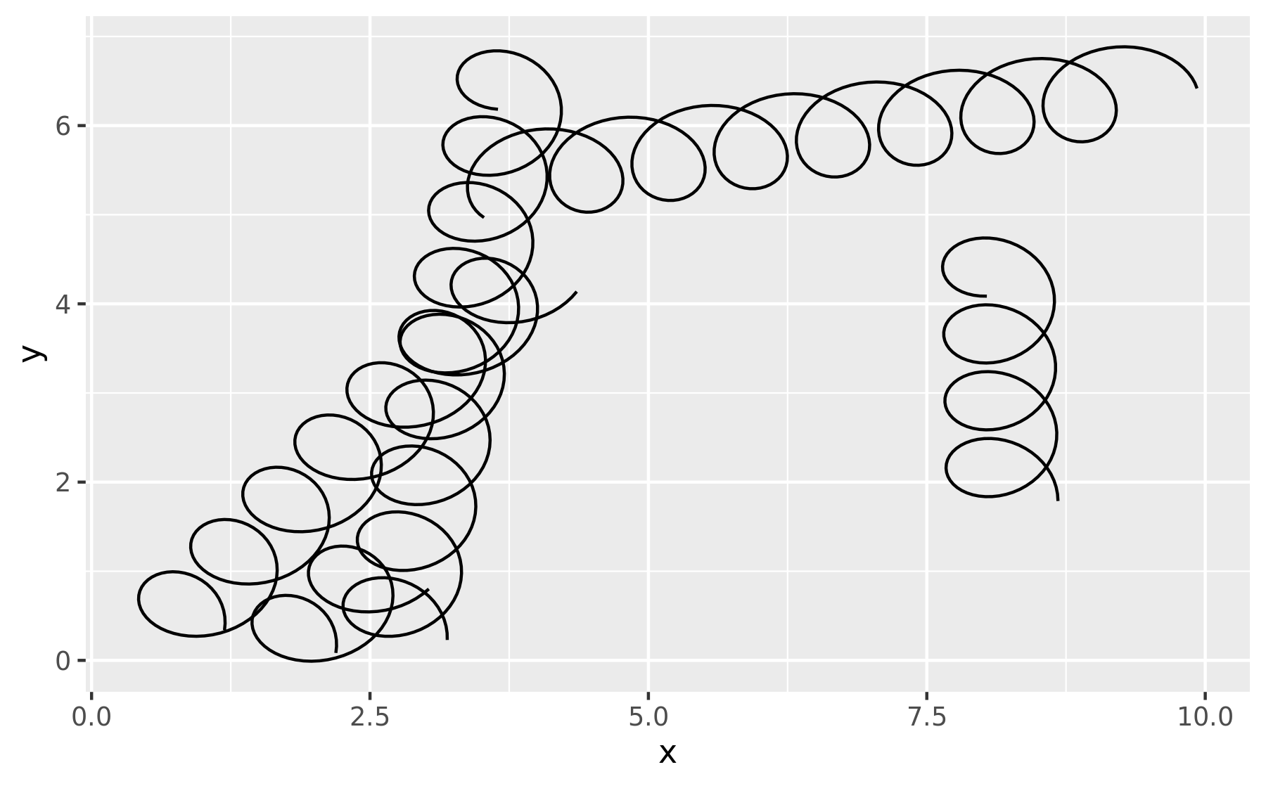
Because we’ve written a new stat, we get a number of features, like scaling and faceting, for free:
ggplot(some_data) +
  geom_spring(
    aes(x, y, xend = xend, yend = yend, colour = class),
    size = 1
  ) +
  facet_wrap(~ class)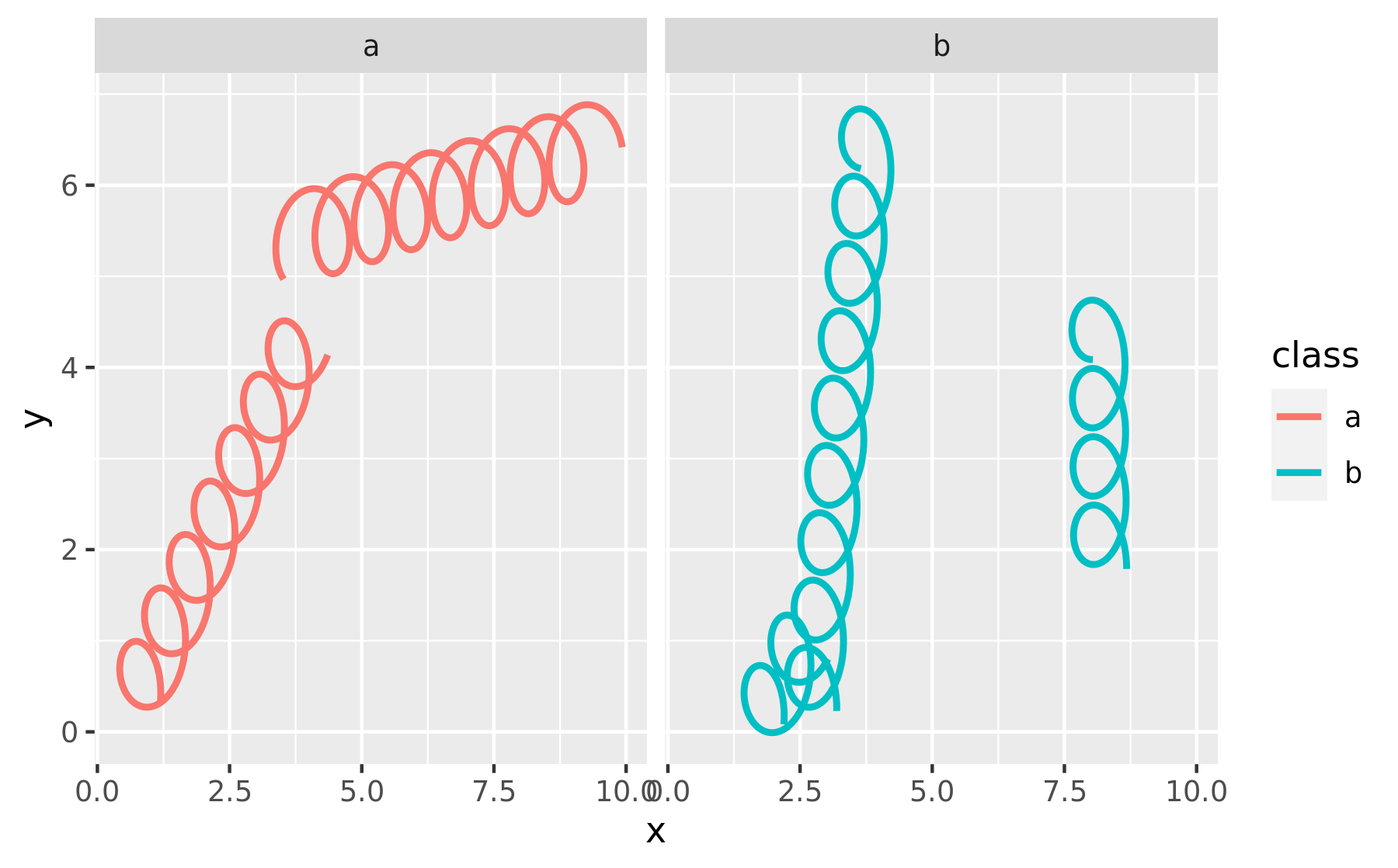
For completion you should also create a stat constructor.
Here our stat_spring() is very similar to geom_spring() except that it provides a default geom instead of a default stat.
stat_spring <- function(mapping = NULL, data = NULL, geom = "path",
                        position = "identity", ..., diameter = 1, tension = 0.75,
                        n = 50, na.rm = FALSE, show.legend = NA,
                        inherit.aes = TRUE) {
  layer(
    data = data,
    mapping = mapping,
    stat = StatSpring,
    geom = geom,
    position = position,
    show.legend = show.legend,
    inherit.aes = inherit.aes,
    params = list(
      diameter = diameter,
      tension = tension,
      n = n,
      na.rm = na.rm,
      ...
    )
  )
}
We can test it out by drawing our springs with dots:
ggplot(some_data) +
  stat_spring(
    aes(x, y, xend = xend, yend = yend, colour = class),
    geom = 'point',
    n = 15
  ) +
  facet_wrap(~ class)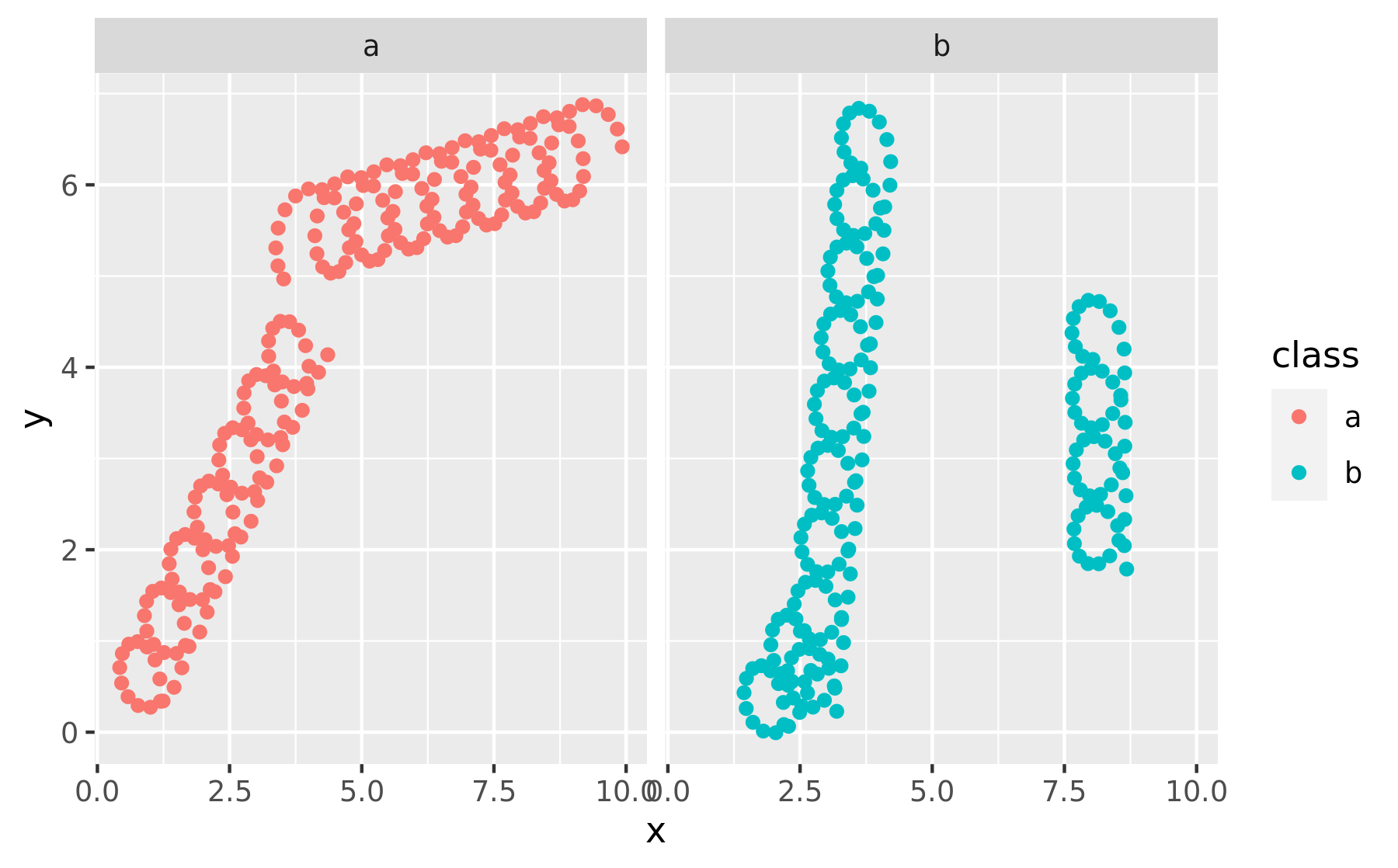
21.2.4 Post-mortem
We have now successfully created our first extension. One shortcoming of our implementation is that diameter and tension are constants that can only be set for the full layer. These settings feel more like aesthetics and it would be nice if their values could be mapped to a variable in the data.
Another, potentially bigger, issue is that the spring path is relative to the coordinate system of the plot. This means that strong deviations from an aspect ratio of 1 will visibly distort the spring, as can be seen in the example below:
ggplot() +
  geom_spring(aes(x = 0, y = 0, xend = 3, yend = 20))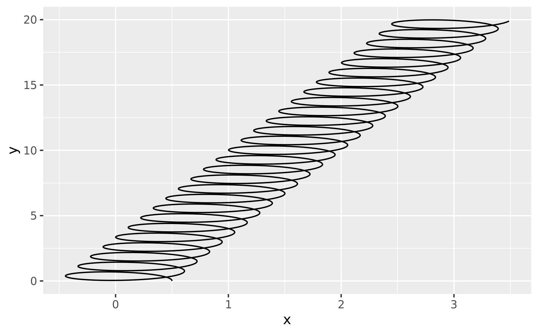
The same underlying problem means that the diameter is expressed in coordinate space, meaning that it is difficult to define a meaningful default:
ggplot() +
  geom_spring(aes(x = 0, y = 0, xend = 100, yend = 80))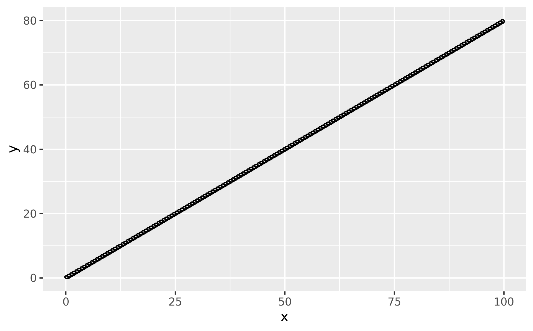
You can also choose to extend an existing
Statclass, but that is relatively uncommon.↩︎