2.7 Modifying the axes

You’ll learn the full range of options available in Chapter ??, but two families of useful helpers let you make the most common modifications. xlab() and ylab() modify the x- and y-axis labels:

ggplot(mpg, aes(cty, hwy)) +
  geom_point(alpha = 1 / 3)

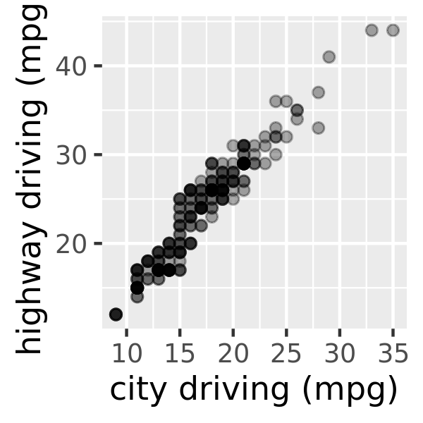
ggplot(mpg, aes(cty, hwy)) +
  geom_point(alpha = 1 / 3) + 
  xlab("city driving (mpg)") + 
  ylab("highway driving (mpg)")

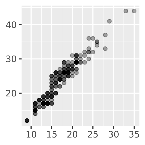
# Remove the axis labels with NULL
ggplot(mpg, aes(cty, hwy)) +
  geom_point(alpha = 1 / 3) + 
  xlab(NULL) + 
  ylab(NULL)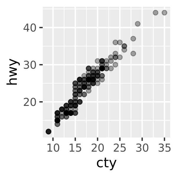

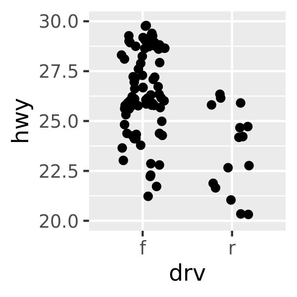
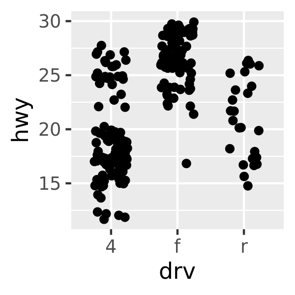
xlim() and ylim() modify the limits of axes:

ggplot(mpg, aes(drv, hwy)) +
  geom_jitter(width = 0.25)

ggplot(mpg, aes(drv, hwy)) +
  geom_jitter(width = 0.25) + 
  xlim("f", "r") + 
  ylim(20, 30)
#> Warning: Removed 138 rows containing missing values (geom_point).
  
# For continuous scales, use NA to set only one limit
ggplot(mpg, aes(drv, hwy)) +
  geom_jitter(width = 0.25, na.rm = TRUE) + 
  ylim(NA, 30)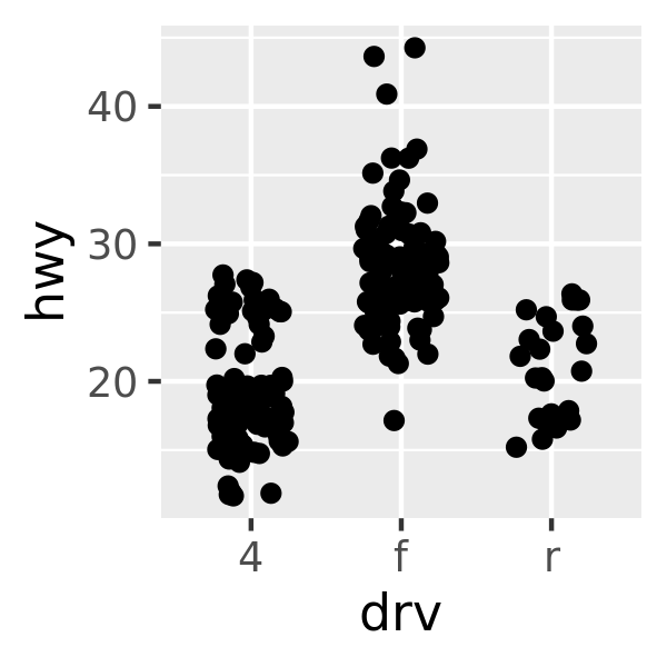

Changing the axes limits sets values outside the range to NA. You can suppress the associated warning with na.rm = TRUE, but be careful. If your plot calculates summary statistics (e.g., sample mean), this conversion to NA occurs before the summary statistics are computed, and may lead to undesirable results in some situations.