9.3 Discrete

It is also possible to map discrete variables to position scales, with the default scales being scale_x_discrete() and scale_y_discrete() in this case. For example, the following two plot specifications are equivalent

ggplot(mpg, aes(x = hwy, y = class)) + 
  geom_point()

ggplot(mpg, aes(x = hwy, y = class)) + 
  geom_point() + 
  scale_x_continuous() +
  scale_y_discrete()

Internally, ggplot2 handles discrete scales by mapping each category to an integer value and then drawing the geom at the corresponding coordinate location. To illustrate this, we can add a custom annotation (see Section 7.4) to the plot:

ggplot(mpg, aes(x = hwy, y = class)) + 
  geom_point() +
  annotate("text", x = 5, y = 1:7, label = 1:7)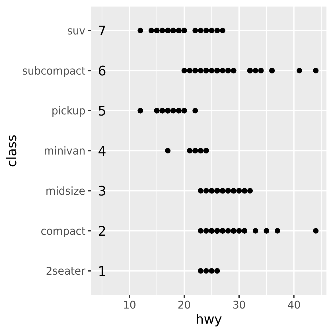

9.3.1 Limits

• For discrete scales, limits should be a character vector that enumerates all possible values.

9.3.2 Scale labels

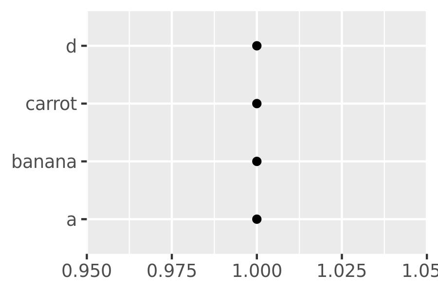
When the data are categorical, you also have the option of using a named vector to set the labels associated with particular values. This allows you to change some labels and not others, without altering the ordering or the breaks:

base <- ggplot(toy, aes(const, txt)) + 
  geom_point() +
  labs(x = NULL, y = NULL)

base
base + scale_y_discrete(labels = c(c = "carrot", b = "banana"))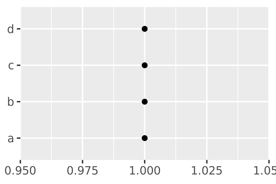

The also contains functions relevant for other kinds of data, such as scales::label_wrap() which allows you to wrap long strings across lines.

9.3.3 guide_axis()

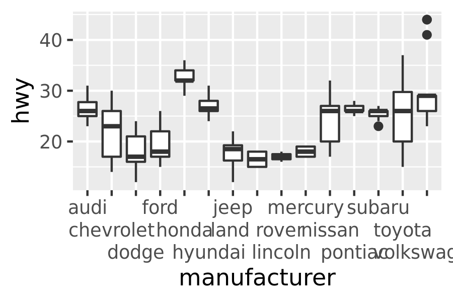
Guide functions exist mostly to control plot legends, but—as legends and axes are both kinds of guide—ggplot2 also supplies a guide_axis() function for axes. Its main purpose is to provide additional controls that prevent labels from overlapping:

base <- ggplot(mpg, aes(manufacturer, hwy)) + geom_boxplot() 

base + guides(x = guide_axis(n.dodge = 3))
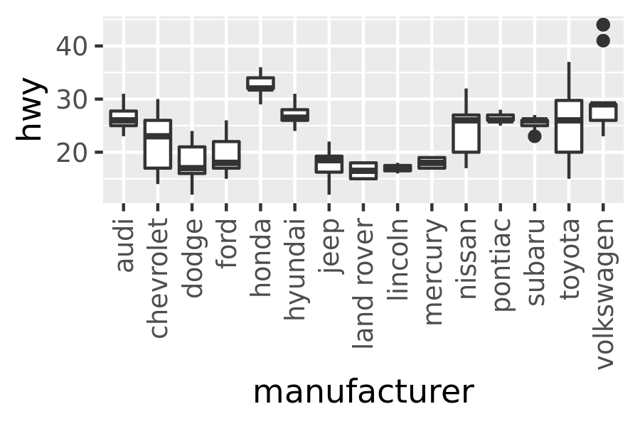
base + guides(x = guide_axis(angle = 90))