16 Faceting

You first encountered faceting in Section 2.5. Faceting generates small multiples each showing a different subset of the data. Small multiples are a powerful tool for exploratory data analysis: you can rapidly compare patterns in different parts of the data and see whether they are the same or different. This section will discuss how you can fine-tune facets, particularly the way in which they interact with position scales.

There are three types of faceting:

• facet_null(): a single plot, the default.

• facet_wrap(): “wraps” a 1d ribbon of panels into 2d.

• facet_grid(): produces a 2d grid of panels defined by variables which form the rows and columns.

The differences between facet_wrap() and facet_grid() are illustrated in Figure 16.1.

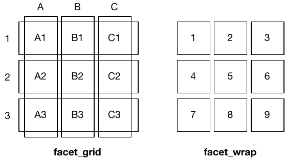
Figure 16.1: A sketch illustrating the difference between the two faceting systems. facet_grid() (left) is fundamentally 2d, being made up of two independent components. facet_wrap() (right) is 1d, but wrapped into 2d to save space.

Faceted plots have the capability to fill up a lot of space, so for this chapter we will use a subset of the mpg dataset that has a manageable number of levels: three cylinders (4, 6, 8), two types of drive train (4 and f), and six classes.

mpg2 <- subset(mpg, cyl != 5 & drv %in% c("4", "f") & class != "2seater")