18.4 Plot functions

Creating small reusable components is most in line with the ggplot2 spirit: you can recombine them flexibly to create whatever plot you want. But sometimes you’re creating the same plot over and over again, and you don’t need that flexibility. Instead of creating components, you might want to write a function that takes data and parameters and returns a complete plot.

For example, you could wrap up the complete code needed to make a piechart:

piechart <- function(data, mapping) {
  ggplot(data, mapping) +
    geom_bar(width = 1) + 
    coord_polar(theta = "y") + 
    xlab(NULL) + 
    ylab(NULL)
}
piechart(mpg, aes(factor(1), fill = class))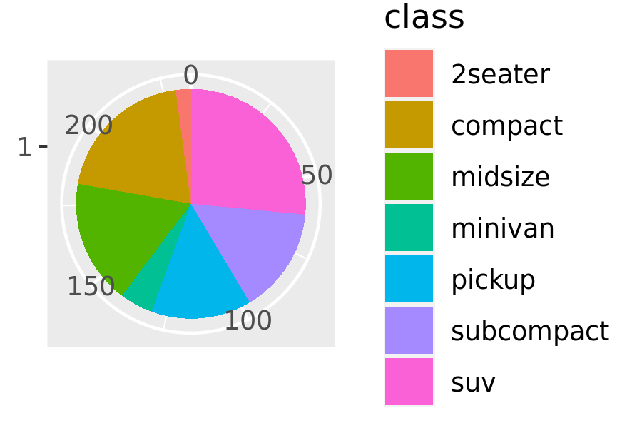

This is much less flexible than the component based approach, but equally, it’s much more concise. Note that I was careful to return the plot object, rather than printing it. That makes it possible add on other ggplot2 components.

You can take a similar approach to drawing parallel coordinates plots (PCPs). PCPs require a transformation of the data, so I recommend writing two functions: one that does the transformation and one that generates the plot. Keeping these two pieces separate makes life much easier if you later want to reuse the same transformation for a different visualisation.

pcp_data <- function(df) {
  is_numeric <- vapply(df, is.numeric, logical(1))

  # Rescale numeric columns
  rescale01 <- function(x) {
    rng <- range(x, na.rm = TRUE)
    (x - rng[1]) / (rng[2] - rng[1])
  }
  df[is_numeric] <- lapply(df[is_numeric], rescale01)
  
  # Add row identifier
  df$.row <- rownames(df)
  
  # Treat numerics as value (aka measure) variables
  # gather_ is the standard-evaluation version of gather, and
  # is usually easier to program with.
  tidyr::gather_(df, "variable", "value", names(df)[is_numeric])
}
pcp <- function(df, ...) {
  df <- pcp_data(df)
  ggplot(df, aes(variable, value, group = .row)) + geom_line(...)
}
pcp(mpg)
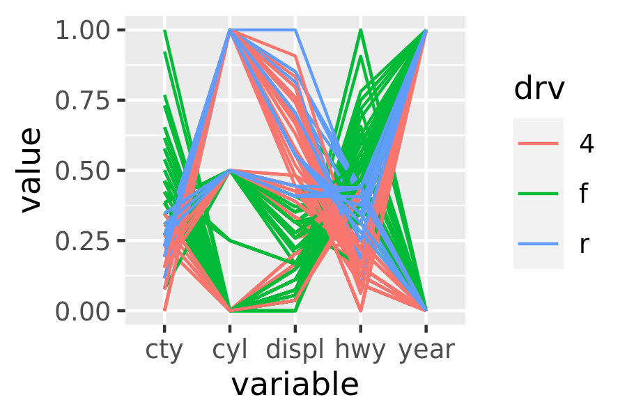
pcp(mpg, aes(colour = drv))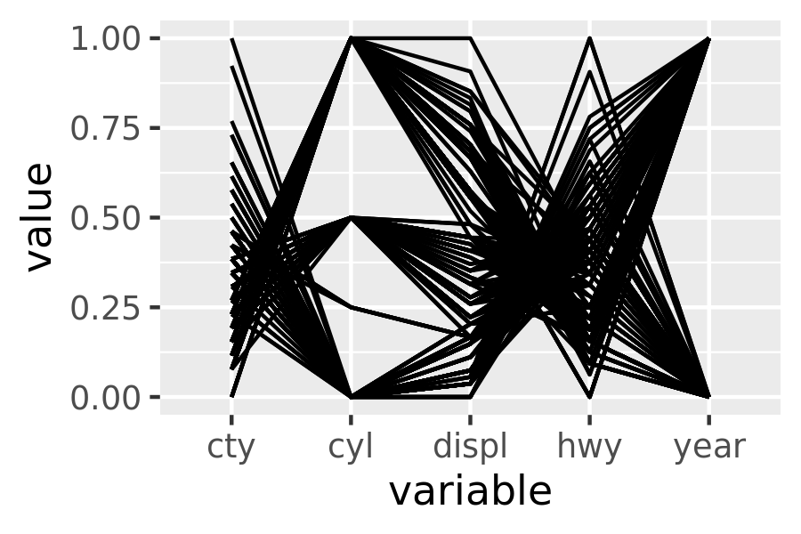

18.4.1 Indirectly referring to variables

The piechart() function above is a little unappealing because it requires the user to know the exact aes() specification that generates a pie chart. It would be more convenient if the user could simply specify the name of the variable to plot. To do that you’ll need to learn a bit more about how aes() works.

aes() uses non-standard evaluation: rather than looking at the values of its arguments, it looks at their expressions. This makes it difficult to work with programmatically as there’s no way to store the name of a variable in an object and then refer to it later:

x_var <- "displ"
aes(x_var)
#> Aesthetic mapping: 
#> * `x` -> `x_var`

Instead we need to use aes_(), which uses regular evaluation. There are two basic ways to create a mapping with aes_():

Using a quoted call, created by quote(), substitute(), as.name(), or parse().

aes_(quote(displ))
#> Aesthetic mapping: 
#> * `x` -> `displ`
aes_(as.name(x_var))
#> Aesthetic mapping: 
#> * `x` -> `displ`
aes_(parse(text = x_var)[[1]])
#> Aesthetic mapping: 
#> * `x` -> `displ`

f <- function(x_var) {
  aes_(substitute(x_var))
}
f(displ)
#> Aesthetic mapping: 
#> * `x` -> `displ`

The difference between as.name() and parse() is subtle. If x_var is “a + b”, as.name() will turn it into a variable called `a + b`, parse() will turn it into the function call a + b. (If this is confusing, http://adv-r.had.co.nz/Expressions.html might help).

Using a formula, created with ~.

aes_(~displ)
#> Aesthetic mapping: 
#> * `x` -> `displ`

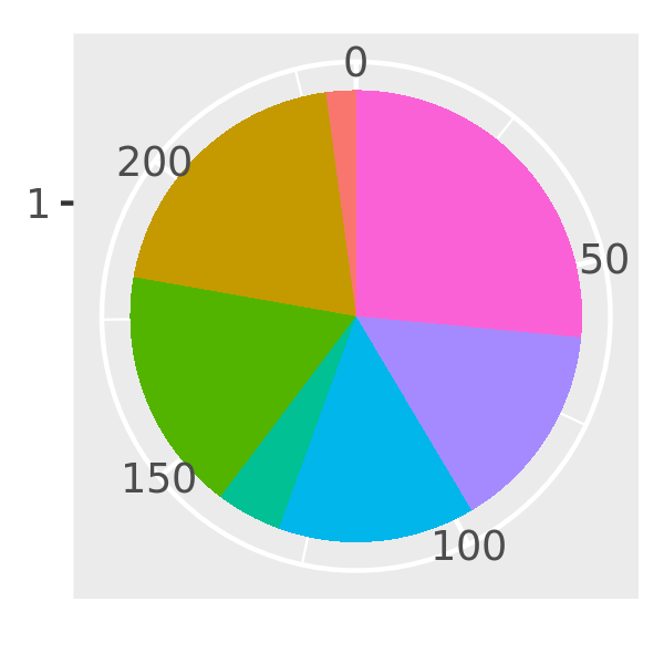
aes_() gives us three options for how a user can supply variables: as a string, as a formula, or as a bare expression. These three options are illustrated below

piechart1 <- function(data, var, ...) {
  piechart(data, aes_(~factor(1), fill = as.name(var)))
}
piechart1(mpg, "class") + theme(legend.position = "none")

piechart2 <- function(data, var, ...) {
  piechart(data, aes_(~factor(1), fill = var))
}
piechart2(mpg, ~class) + theme(legend.position = "none")

piechart3 <- function(data, var, ...) {
  piechart(data, aes_(~factor(1), fill = substitute(var)))
}
piechart3(mpg, class) + theme(legend.position = "none")

There’s another advantage to aes_() over aes() if you’re writing ggplot2 plots inside a package: using aes_(~x, ~y) instead of aes(x, y) avoids the global variables NOTE in R CMD check.

18.4.2 The plot environment

As you create more sophisticated plotting functions, you’ll need to understand a bit more about ggplot2’s scoping rules. ggplot2 was written well before I understood the full intricacies of non-standard evaluation, so it has a rather simple scoping system. If a variable is not found in the data, it is looked for in the plot environment. There is only one environment for a plot (not one for each layer), and it is the environment in which ggplot() is called from (i.e. the parent.frame()).

This means that the following function won’t work because n is not stored in an environment accessible when the expressions in aes() are evaluated.

f <- function() {
  n <- 10
  geom_line(aes(x / n)) 
}
df <- data.frame(x = 1:3, y = 1:3)
ggplot(df, aes(x, y)) + f()

Note that this is only a problem with the mapping argument. All other arguments are evaluated immediately so their values (not a reference to a name) are stored in the plot object. This means the following function will work:

f <- function() {
  colour <- "blue"
  geom_line(colour = colour) 
}
ggplot(df, aes(x, y)) + f()

If you need to use a different environment for the plot, you can specify it with the environment argument to ggplot(). You’ll need to do this if you’re creating a plot function that takes user provided data.

18.4.3 Exercises

Create a distribution() function specially designed for visualising continuous distributions. Allow the user to supply a dataset and the name of a variable to visualise. Let them choose between histograms, frequency polygons, and density plots. What other arguments might you want to include?
What additional arguments should pcp() take? What are the downsides of how ... is used in the current code?

Advanced: why doesn’t this code work? How can you fix it?

f <- function() {
  levs <- c("2seater", "compact", "midsize", "minivan", "pickup", 
    "subcompact", "suv")
  piechart3(mpg, factor(class, levels = levs))
}
f()
#> Error in factor(class, levels = levs): object 'levs' not found