13.5 Geoms

Geometric objects, or geoms for short, perform the actual rendering of the layer, controlling the type of plot that you create. For example, using a point geom will create a scatterplot, while using a line geom will create a line plot.

• Graphical primitives:
  • geom_blank(): display nothing. Most useful for adjusting axes limits using data.
  • geom_point(): points.
  • geom_path(): paths.
  • geom_ribbon(): ribbons, a path with vertical thickness.
  • geom_segment(): a line segment, specified by start and end position.
  • geom_rect(): rectangles.
  • geom_polygon(): filled polygons.
  • geom_text(): text.
• One variable:
  • Discrete:
    • geom_bar(): display distribution of discrete variable.
  • Continuous
    • geom_histogram(): bin and count continuous variable, display with bars.
    • geom_density(): smoothed density estimate.
    • geom_dotplot(): stack individual points into a dot plot.
    • geom_freqpoly(): bin and count continuous variable, display with lines.
• Two variables:
  • Both continuous:
    • geom_point(): scatterplot.
    • geom_quantile(): smoothed quantile regression.
    • geom_rug(): marginal rug plots.
    • geom_smooth(): smoothed line of best fit.
    • geom_text(): text labels.
  • Show distribution:
    • geom_bin2d(): bin into rectangles and count.
    • geom_density2d(): smoothed 2d density estimate.
    • geom_hex(): bin into hexagons and count.
  • At least one discrete:
    • geom_count(): count number of point at distinct locations
    • geom_jitter(): randomly jitter overlapping points.
  • One continuous, one discrete:
    • geom_bar(stat = "identity"): a bar chart of precomputed summaries.
    • geom_boxplot(): boxplots.
    • geom_violin(): show density of values in each group.
  • One time, one continuous
    • geom_area(): area plot.
    • geom_line(): line plot.
    • geom_step(): step plot.
  • Display uncertainty:
    • geom_crossbar(): vertical bar with center.
    • geom_errorbar(): error bars.
    • geom_linerange(): vertical line.
    • geom_pointrange(): vertical line with center.
  • Spatial
    • geom_map(): fast version of geom_polygon() for map data.
• Three variables:
  • geom_contour(): contours.
  • geom_tile(): tile the plane with rectangles.
  • geom_raster(): fast version of geom_tile() for equal sized tiles.

Each geom has a set of aesthetics that it understands, some of which must be provided. For example, the point geoms requires x and y position, and understands colour, size and shape aesthetics. A bar requires height (ymax), and understands width, border colour and fill colour. Each geom lists its aesthetics in the documentation.

Some geoms differ primarily in the way that they are parameterised. For example, you can draw a square in three ways:

• By giving geom_tile() the location (x and y) and dimensions (width and height).

• By giving geom_rect() top (ymax), bottom (ymin), left (xmin) and right (xmax) positions.

• By giving geom_polygon() a four row data frame with the x and y positions of each corner.

Other related geoms are:

• geom_segment() and geom_line()
• geom_area() and geom_ribbon().

If alternative parameterisations are available, picking the right one for your data will usually make it much easier to draw the plot you want.

13.5.1 Exercises

1. Download and print out the ggplot2 cheatsheet from http://www.rstudio.com/resources/cheatsheets/ so you have a handy visual reference for all the geoms.

2. Look at the documentation for the graphical primitive geoms. Which aesthetics do they use? How can you summarise them in a compact form?

3. What’s the best way to master an unfamiliar geom? List three resources to help you get started.

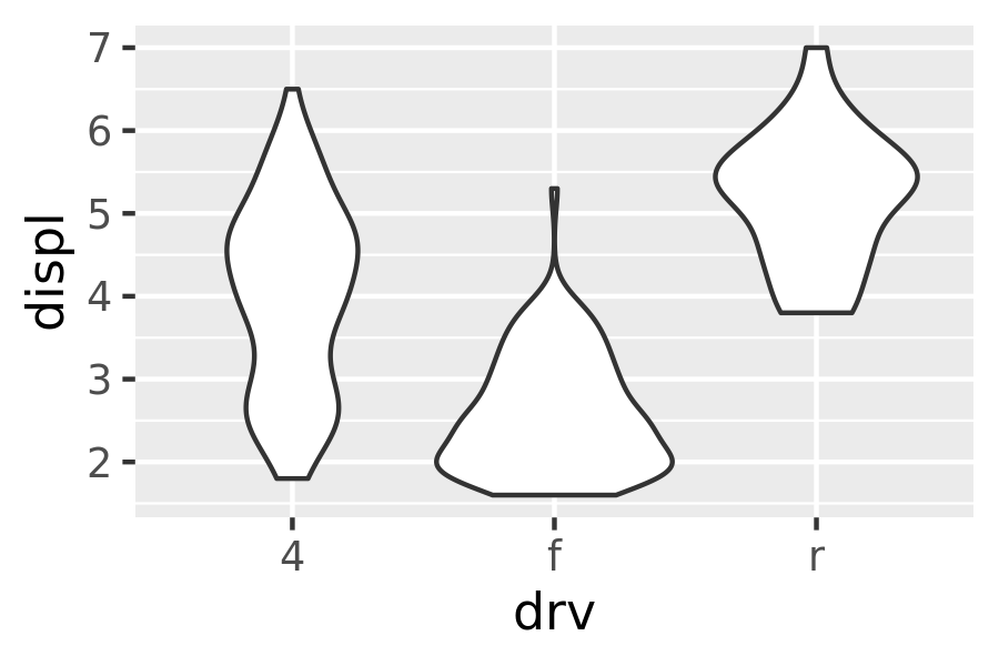
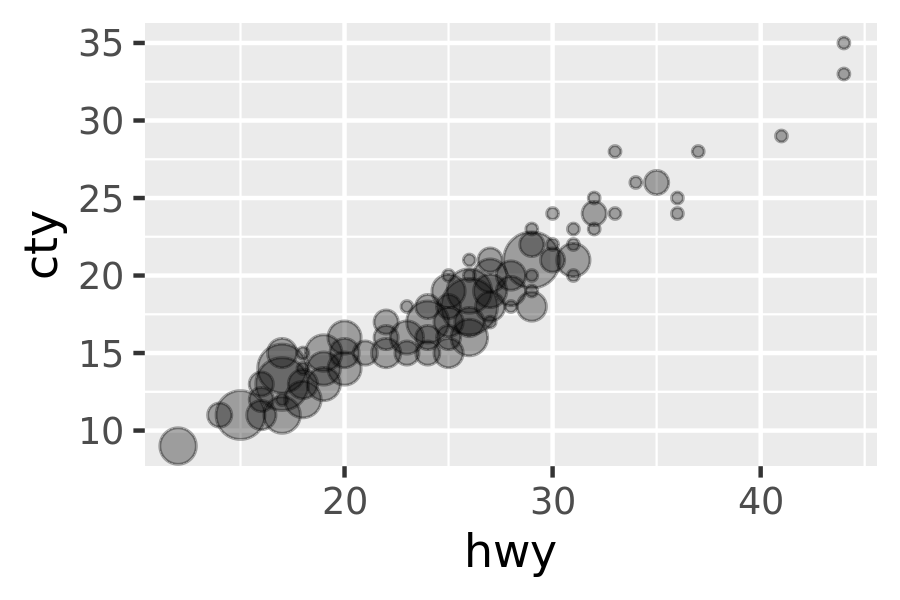
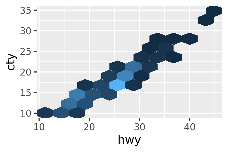
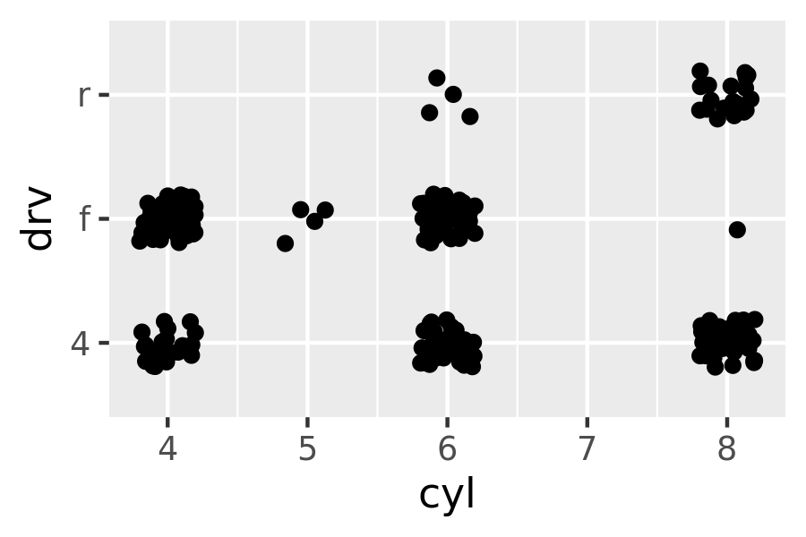
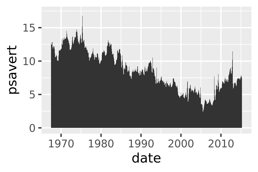
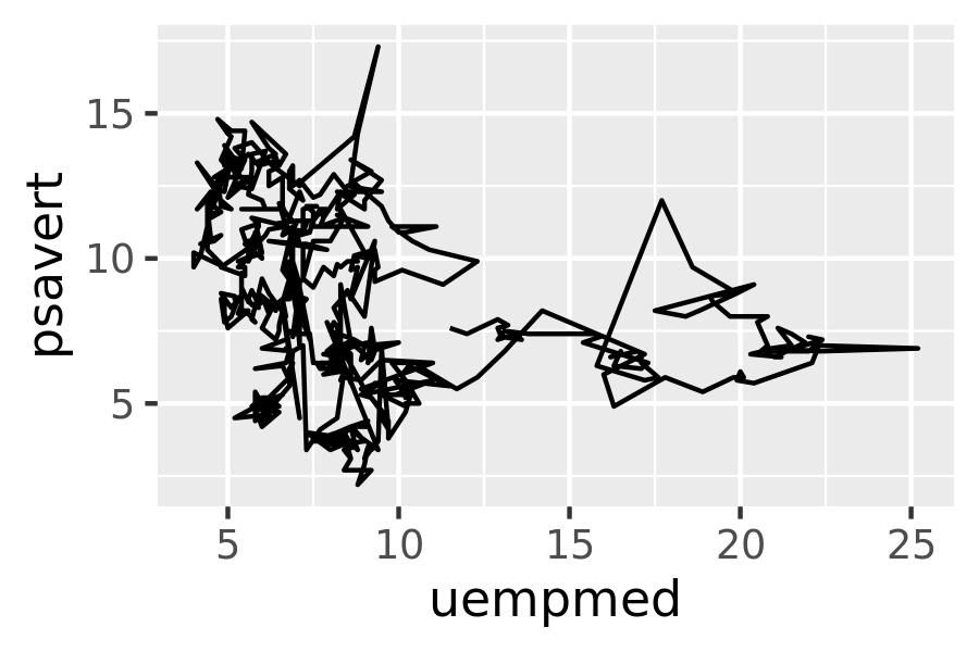
4. For each of the plots below, identify the geom used to draw it.

   

   

   

5. For each of the following problems, suggest a useful geom:

   • Display how a variable has changed over time.
   • Show the detailed distribution of a single variable.
   • Focus attention on the overall trend in a large dataset.
   • Draw a map.
   • Label outlying points.