19.3 The gtable step
The purpose of ggplot_gtable() is to take the output of the build step and turn it into a single gtable object that can be plotted using grid. At this point the main elements responsible for further computations are the geoms, the coordinate system, the facet, and the theme. The stats and position adjustments have all played their part already.
19.3.1 Rendering the panels
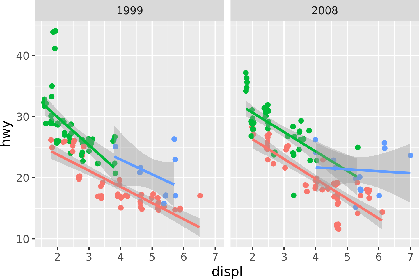
The first thing that happens is that the data is converted into its graphical representation. This happens in two steps. First, each layer is converted into a list of graphical objects (grobs). As with stats the conversion happens by splitting the data, first by PANEL, and then by group, with the possibility of the geom intercepting this splitting for performance reasons. While a lot of the data preparation has been performed already it is not uncommon that the geom does some additional transformation of the data during this step. A crucial part is to transform and normalise the position data. This is done by the coordinate system and while it often simply means that the data is normalised based on the limits of the coordinate system, it can also include radical transformations such as converting the positions into polar coordinates. The output of this is for each layer a list of gList objects corresponding to each panel in the facet layout. After this the facet takes over and assembles the panels. It does this by first collectiong the grobs for each panel from the layers, along with rendering strips, backgrounds, gridlines,and axes based on the theme and combines all of this into a single gList for each panel. It then proceeds to arranging all these panels into a gtable based on the calculated panel layout. For most plots this is simple as there is only a single panel, but for e.g. plots using facet_wrap() it can be quite complicated. The output is the basis of the final gtable object. At this stage in the process our example plot p looks like this:
19.3.2 Adding guides
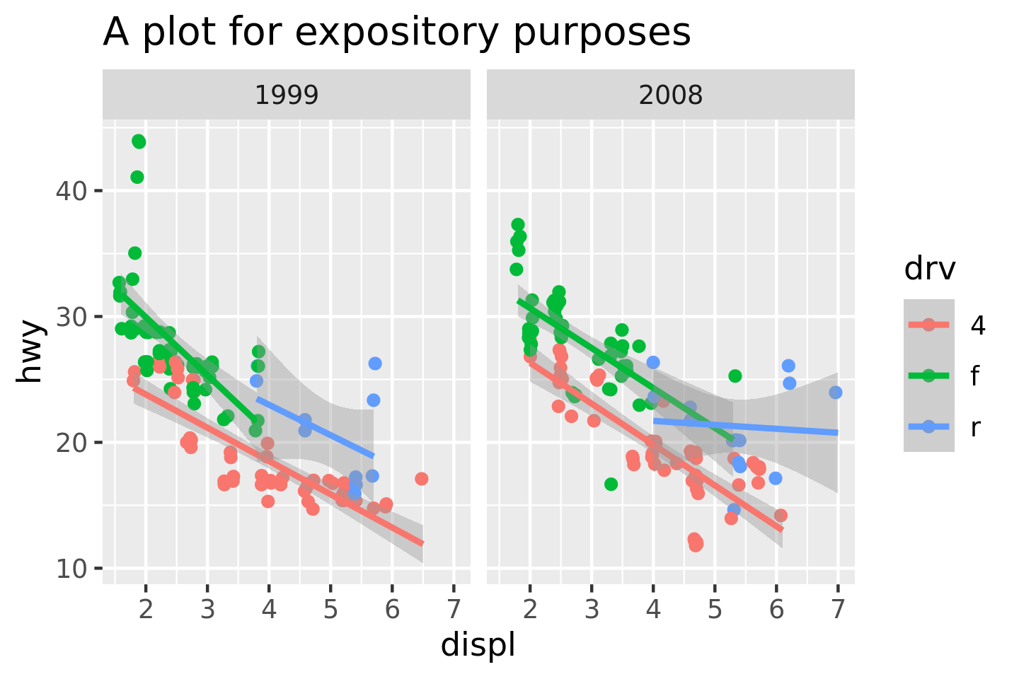
There are two types of guides in ggplot2: axes and legends. As our plot p illustrates at this point the axes has already been rendered and assembled together with the panels, but the legends are still missing. Rendering the legends is a complicated process that first trains a guide for each scale. Then, potentially multiple guides are merged if their mapping allows it before the layers that contribute to the legend is asked for key grobs for each key in the legend. These key grobs are then assembled across layers and combined to the final legend in a process that is quite reminiscent of how layers gets combined into the gtable of panels. In the end the output is a gtable that holds each legend box arranged and styled according to the theme and guide specifications. Once created the guide gtable is then added to the main gtable according to the legend.position theme setting. At this stage, our example plot is complete in most respects: the only thing missing is the title.
19.3.3 Adding adornment
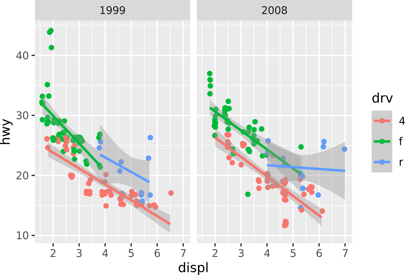
The only thing remaining is to add title, subtitle, caption, and tag as well as add background and margins, at which point the final gtable is done.
19.3.4 Output
At this point ggplot2 is ready to hand over to grid. Our rendering process is more or less equivalent to the code below and the end result is, as described above, a gtable:
p_built <- ggplot_build(p)
p_gtable <- ggplot_gtable(p_built)

class(p_gtable)
#> [1] "gtable" "gTree"  "grob"   "gDesc"
What is less obvious is that the dimensions of the object is unpredictable and will depend on both the faceting, legend placement, and which titles are drawn. It is thus not advised to depend on row and column placement in your code, should you want to further modify the gtable. All elements of the gtable are named though, so it is still possible to reliably retrieve, e.g. the grob holding the top-left y-axis with a bit of work. As an illustration, the gtable for our plot p is shown in the code below:
p_gtable
#> TableGrob (13 x 15) "layout": 22 grobs
#>     z         cells        name                                          grob
#> 1   0 ( 1-13, 1-15)  background               rect[plot.background..rect.741]
#> 2   1 ( 8- 8, 5- 5)   panel-1-1                      gTree[panel-1.gTree.612]
#> 3   1 ( 8- 8, 9- 9)   panel-2-1                      gTree[panel-2.gTree.627]
#> 4   3 ( 6- 6, 5- 5)  axis-t-1-1                                zeroGrob[NULL]
#> 5   3 ( 6- 6, 9- 9)  axis-t-2-1                                zeroGrob[NULL]
#> 6   3 ( 9- 9, 5- 5)  axis-b-1-1           absoluteGrob[GRID.absoluteGrob.631]
#> 7   3 ( 9- 9, 9- 9)  axis-b-2-1           absoluteGrob[GRID.absoluteGrob.631]
#> 8   3 ( 8- 8, 8- 8)  axis-l-1-2                                zeroGrob[NULL]
#> 9   3 ( 8- 8, 4- 4)  axis-l-1-1           absoluteGrob[GRID.absoluteGrob.639]
#> 10  3 ( 8- 8,10-10)  axis-r-1-2                                zeroGrob[NULL]
#> 11  3 ( 8- 8, 6- 6)  axis-r-1-1                                zeroGrob[NULL]
#> 12  2 ( 7- 7, 5- 5) strip-t-1-1                                 gtable[strip]
#> 13  2 ( 7- 7, 9- 9) strip-t-2-1                                 gtable[strip]
#> 14  4 ( 5- 5, 5- 9)      xlab-t                                zeroGrob[NULL]
#> 15  5 (10-10, 5- 9)      xlab-b titleGrob[axis.title.x.bottom..titleGrob.694]
#> 16  6 ( 8- 8, 3- 3)      ylab-l   titleGrob[axis.title.y.left..titleGrob.697]
#> 17  7 ( 8- 8,11-11)      ylab-r                                zeroGrob[NULL]
#> 18  8 ( 8- 8,13-13)   guide-box                             gtable[guide-box]
#> 19  9 ( 4- 4, 5- 9)    subtitle         zeroGrob[plot.subtitle..zeroGrob.737]
#> 20 10 ( 3- 3, 5- 9)       title          titleGrob[plot.title..titleGrob.736]
#> 21 11 (11-11, 5- 9)     caption          zeroGrob[plot.caption..zeroGrob.739]
#> 22 12 ( 2- 2, 2- 2)         tag              zeroGrob[plot.tag..zeroGrob.738]
The final plot, as one would hope, looks identical to the original:
grid::grid.newpage()
grid::grid.draw(p_gtable)