16.5 Grouping vs. faceting

Faceting is an alternative to using aesthetics (like colour, shape or size) to differentiate groups. Both techniques have strengths and weaknesses, based around the relative positions of the subsets. With faceting, each group is quite far apart in its own panel, and there is no overlap between the groups. This is good if the groups overlap a lot, but it does make small differences harder to see. When using aesthetics to differentiate groups, the groups are close together and may overlap, but small differences are easier to see.

df <- data.frame(
  x = rnorm(120, c(0, 2, 4)),
  y = rnorm(120, c(1, 2, 1)),
  z = letters[1:3]
)

ggplot(df, aes(x, y)) + 
  geom_point(aes(colour = z))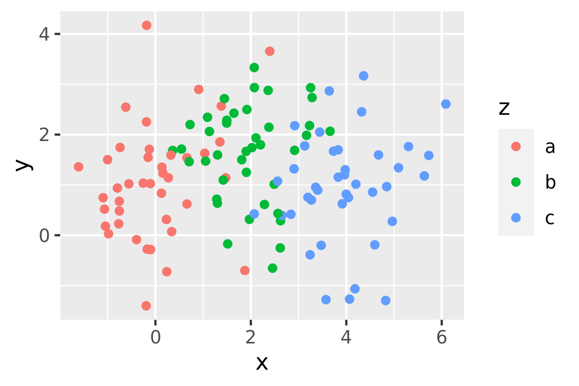

ggplot(df, aes(x, y)) + 
  geom_point() + 
  facet_wrap(~z)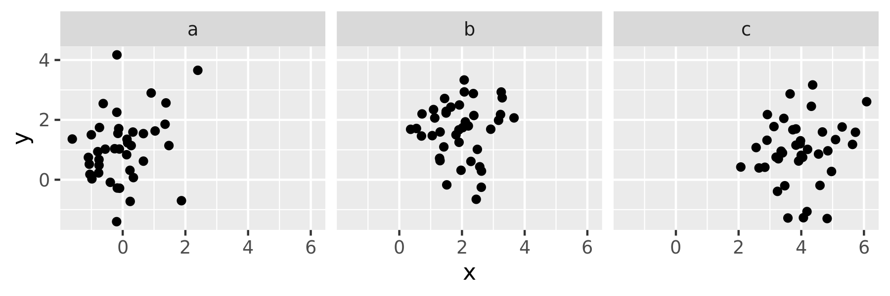

Comparisons between facets often benefit from some thoughtful annotation. For example, in this case we could show the mean of each group in every panel. To do this we group and summarise the data using the dplyr package, which is covered in R for Data Science at https://r4ds.had.co.nz. Note that we need two “z” variables: one for the facets and one for the colours.

df_sum <- df %>% 
  group_by(z) %>% 
  summarise(x = mean(x), y = mean(y)) %>%
  rename(z2 = z)
#> `summarise()` ungrouping output (override with `.groups` argument)
ggplot(df, aes(x, y)) + 
  geom_point() + 
  geom_point(data = df_sum, aes(colour = z2), size = 4) + 
  facet_wrap(~z)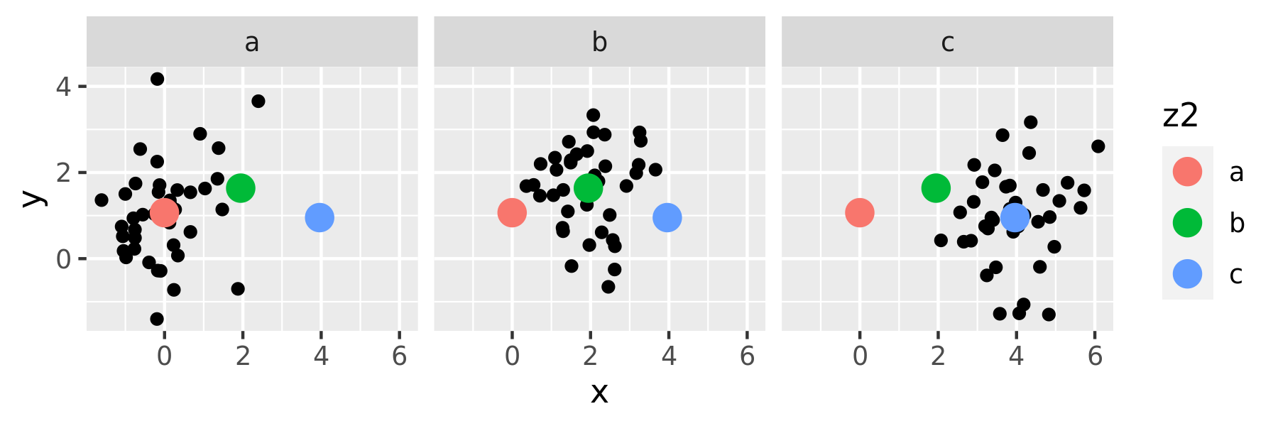

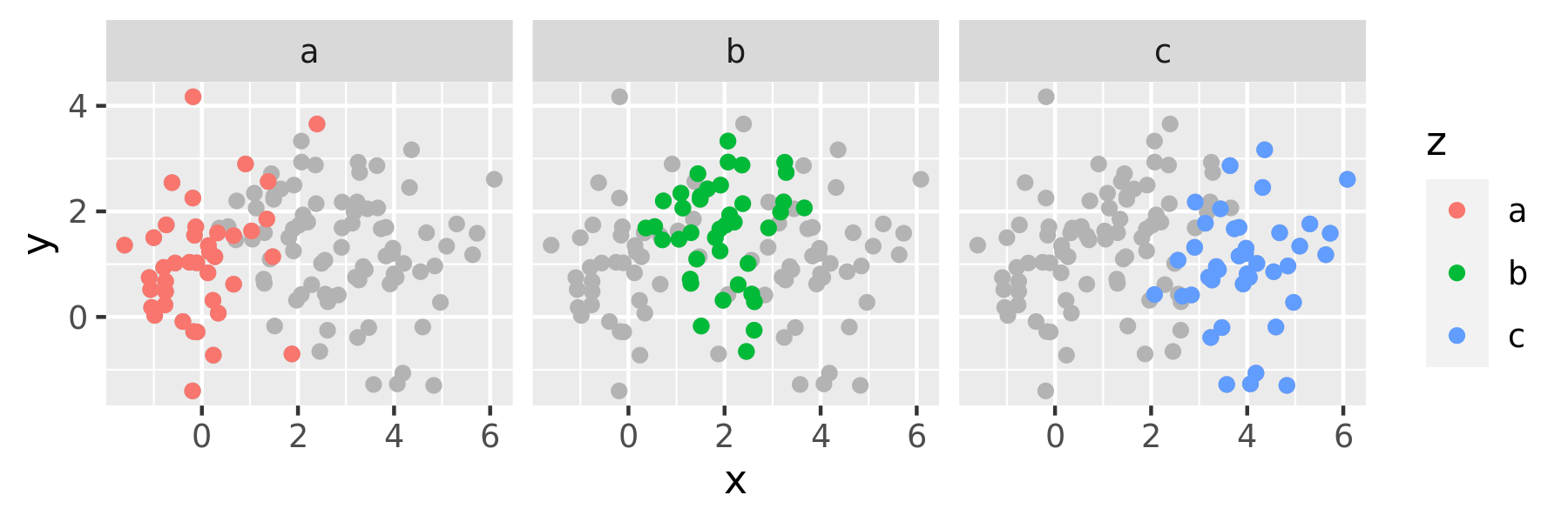
Another useful technique is to put all the data in the background of each panel:

df2 <- dplyr::select(df, -z)

ggplot(df, aes(x, y)) + 
  geom_point(data = df2, colour = "grey70") +
  geom_point(aes(colour = z)) + 
  facet_wrap(~z)