14.5 Legend merging and splitting

There is always a one-to-one correspondence between position scales and axes. But the connection between non-position scales and legend is more complex: one legend may need to draw symbols from multiple layers (“merging”), or one aesthetic may need multiple legends (“splitting”).

14.5.1 Merging legends

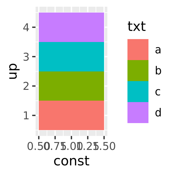
Merging legends occurs quite frequently when using ggplot2. For example, if you’ve mapped colour to both points and lines, the keys will show both points and lines. If you’ve mapped fill colour, you get a rectangle. Note the way the legend varies in the plots below:

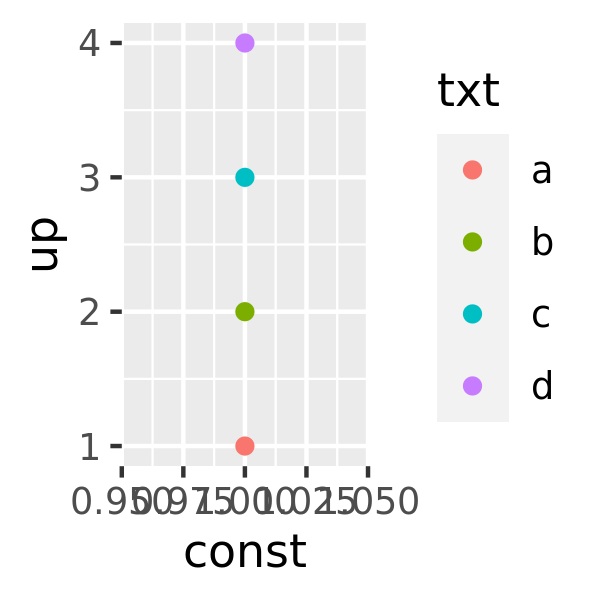
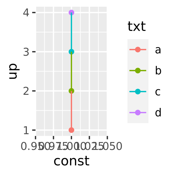
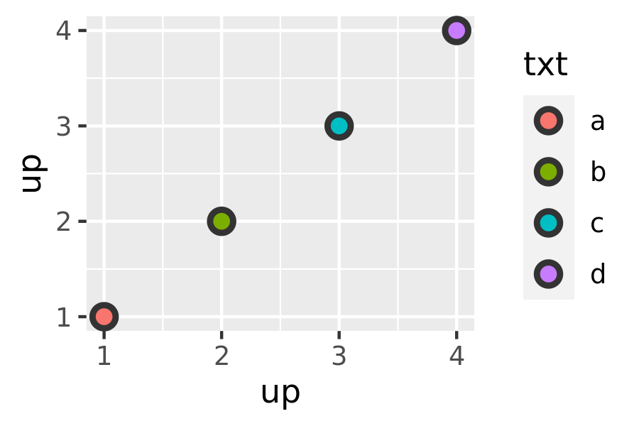
By default, a layer will only appear if the corresponding aesthetic is mapped to a variable with aes(). You can override whether or not a layer appears in the legend with show.legend: FALSE to prevent a layer from ever appearing in the legend; TRUE forces it to appear when it otherwise wouldn’t. Using TRUE can be useful in conjunction with the following trick to make points stand out:

ggplot(toy, aes(up, up)) + 
  geom_point(size = 4, colour = "grey20") +
  geom_point(aes(colour = txt), size = 2) 

ggplot(toy, aes(up, up)) + 
  geom_point(size = 4, colour = "grey20", show.legend = TRUE) +
  geom_point(aes(colour = txt), size = 2)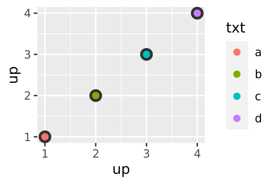

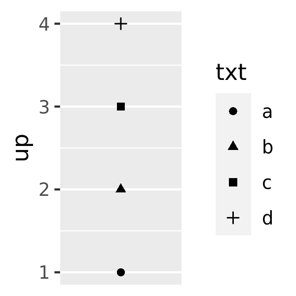
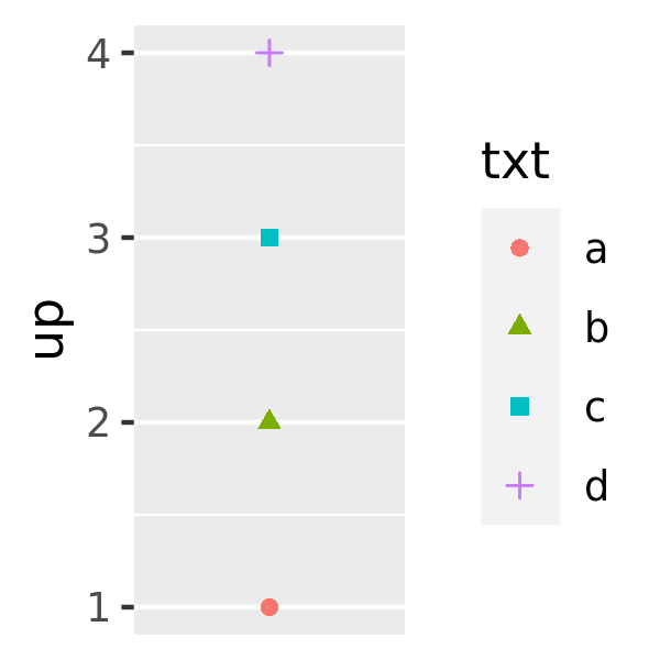
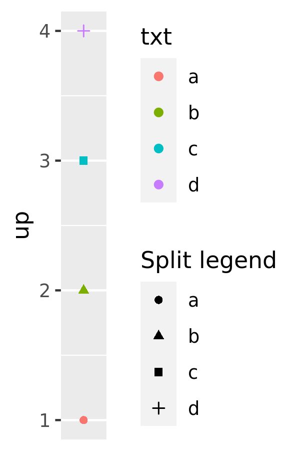
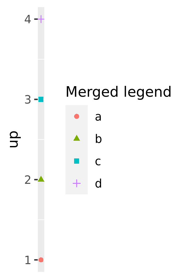
ggplot2 tries to use the fewest number of legends to accurately convey the aesthetics used in the plot. It does this by combining legends where the same variable is mapped to different aesthetics. The figure below shows how this works for points: if both colour and shape are mapped to the same variable, then only a single legend is necessary.

base <- ggplot(toy, aes(const, up)) +
  scale_x_continuous(NULL, breaks = NULL)
base + geom_point(aes(colour = txt))
base + geom_point(aes(shape = txt))
base + geom_point(aes(shape = txt, colour = txt))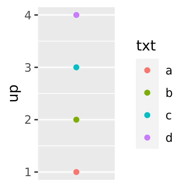

In order for legends to be merged, they must have the same name. So if you change the name of one of the scales, you’ll need to change it for all of them. One way to do this is by using labs() helper function:

base <- ggplot(toy, aes(const, up)) + 
  geom_point(aes(shape = txt, colour = txt)) + 
  scale_x_continuous(NULL, breaks = NULL)

base
base + labs(shape = "Split legend")
base + labs(shape = "Merged legend", colour = "Merged legend")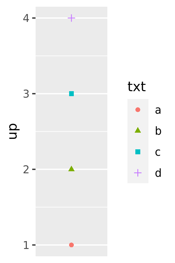

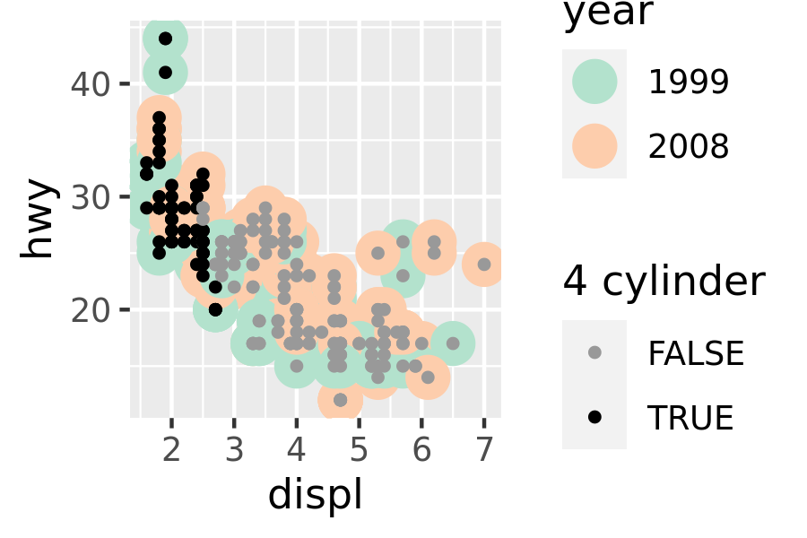
14.5.2 Splitting legends

Splitting a legend is a much less common data visualisation task. In general it is not advisable to map one aesthetic (e.g. colour) to multiple variables, and so by default ggplot2 does not allow you to “split” the colour aesthetic into multiple scales with separate legends. Nevertheless, there are exceptions to this general rule, and it is possible to override this behaviour using the ggnewscale package.⁴³ The ggnewscale::new_scale_colour() command acts as an instruction to ggplot2 to initialise a new colour scale: scale and guide commands that appear above the new_scale_colour() command will be applied to the first colour scale, and commands that appear below are applied to the second colour scale.

To illustrate this the plot on the left uses geom_point() to display a large marker for each vehicle make in the mpg data, with a single colour scale that maps to the year. On the right, a second geom_point() layer is overlaid on the plot using small markers: this layer is associated with a different colour scale, used to indicate whether the vehicle has a 4-cylinder engine.

base <- ggplot(mpg, aes(displ, hwy)) + 
  geom_point(aes(colour = factor(year)), size = 5) + 
  scale_colour_brewer("year", type = "qual", palette = 5) 

base
base + 
  ggnewscale::new_scale_colour() + 
  geom_point(aes(colour = cyl == 4), size = 1, fill = NA) + 
  scale_colour_manual("4 cylinder", values = c("grey60", "black"))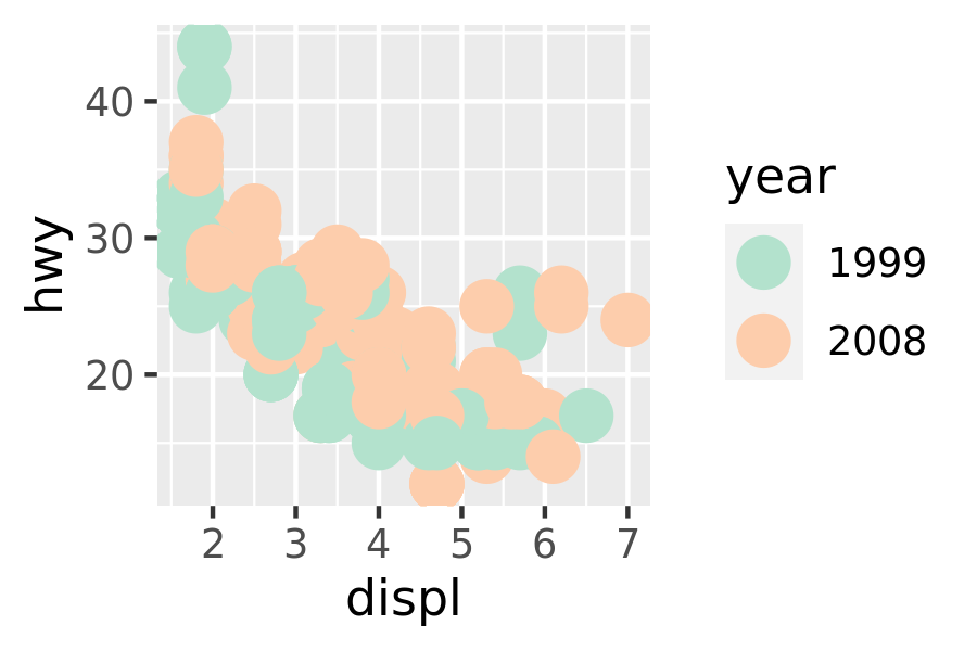

Additional details, including functions that apply to other scale types, are available on the package website, https://github.com/eliocamp/ggnewscale.

Elio Campitelli, Ggnewscale: Multiple Fill and Colour Scales in ’Ggplot2’, 2020, https://CRAN.R-project.org/package=ggnewscale.↩︎