9.5 Limits
All scales have limits that define the domain over which the scale is defined and are usually derived from the range of the data. Here we’ll discuss why you might want to specify the limits rather than relying on the data:
- You want to shrink the limits to focus on an interesting area of the plot.
- You want to expand the limits to make multiple plots match up or to match the natural limits of a variable (e.g. percentages go from 0 to 100).
It’s most natural to think about the limits of position scales: they map directly to the ranges of the axes. But limits also apply to scales that have legends, like colour, size, and shape, and these limits are particularly important if you want colours to be consistent across multiple plots.
Use the limits argument to modify limits:
- For continuous scales,
limitsshould be a numeric vector of length two. If you only want to set the upper or lower limit, you can set the other value toNA.
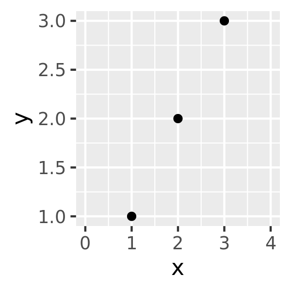
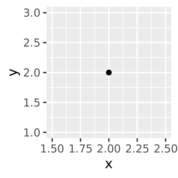
A minimal example is shown below. In the left panel the limits of the x scale are set to the default values (the range of the data), the middle panel expands the limits, and the right panel shrinks them:
df <- data.frame(x = 1:3, y = 1:3)
base <- ggplot(df, aes(x, y)) + geom_point()

base
base + scale_x_continuous(limits = c(0, 4))
base + scale_x_continuous(limits = c(1.5, 2.5))
#> Warning: Removed 2 rows containing missing values (geom_point).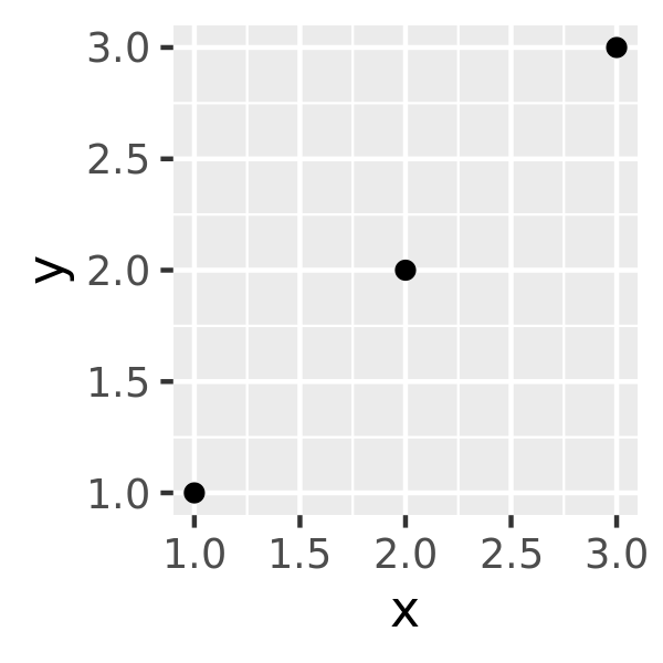
You might be surprised that the final plot generates a warning, as there’s no missing value in the input dataset. I’ll talk about this in Section 9.1.2.
9.5.1 Setting multiple limits
Manually setting scale limits is a common task when you need to ensure that scales in different plots are consistent with one another. When you create a faceted plot, ggplot2 automatically does this for you:
ggplot(mpg, aes(displ, hwy, colour = fl)) +
  geom_point() +
  facet_wrap(vars(year))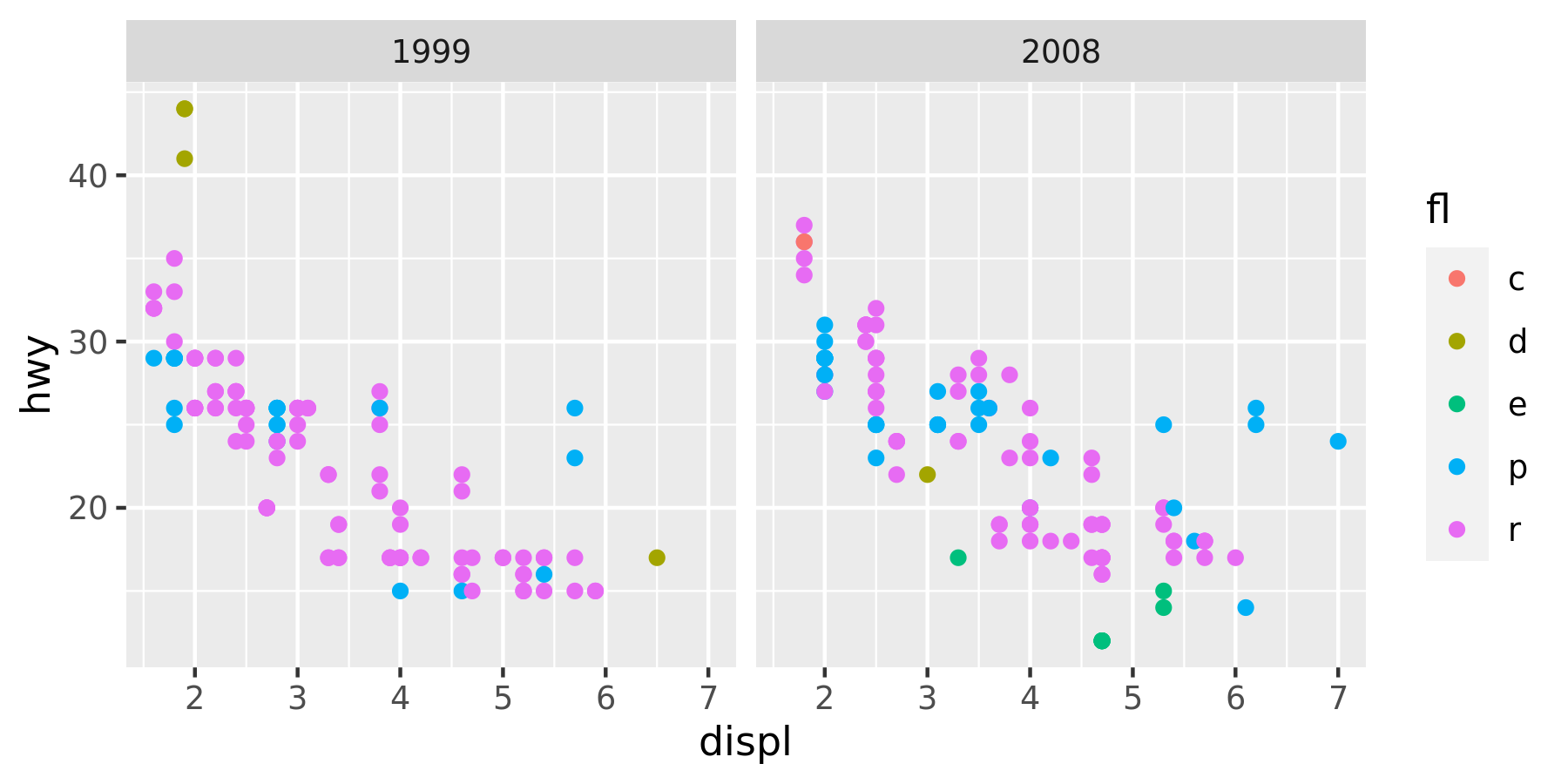
(Colour represents the fuel type, which can be regular, ethanol, diesel, premium or compressed natural gas.)
In this plot the x and y axes have the same limits in both facets and the colours are consistent. However, it is sometimes necessary to maintain consistency across multiple plots, which has the often-undesirable property of causing each plot to set scale limits independently:
mpg_99 <- mpg %>% filter(year == 1999)
mpg_08 <- mpg %>% filter(year == 2008)

base_99 <- ggplot(mpg_99, aes(displ, hwy, colour = fl)) + geom_point()
base_08 <- ggplot(mpg_08, aes(displ, hwy, colour = fl)) + geom_point()

base_99
base_08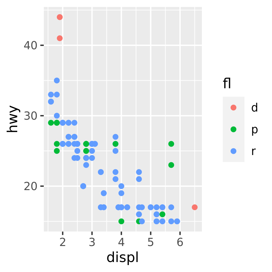
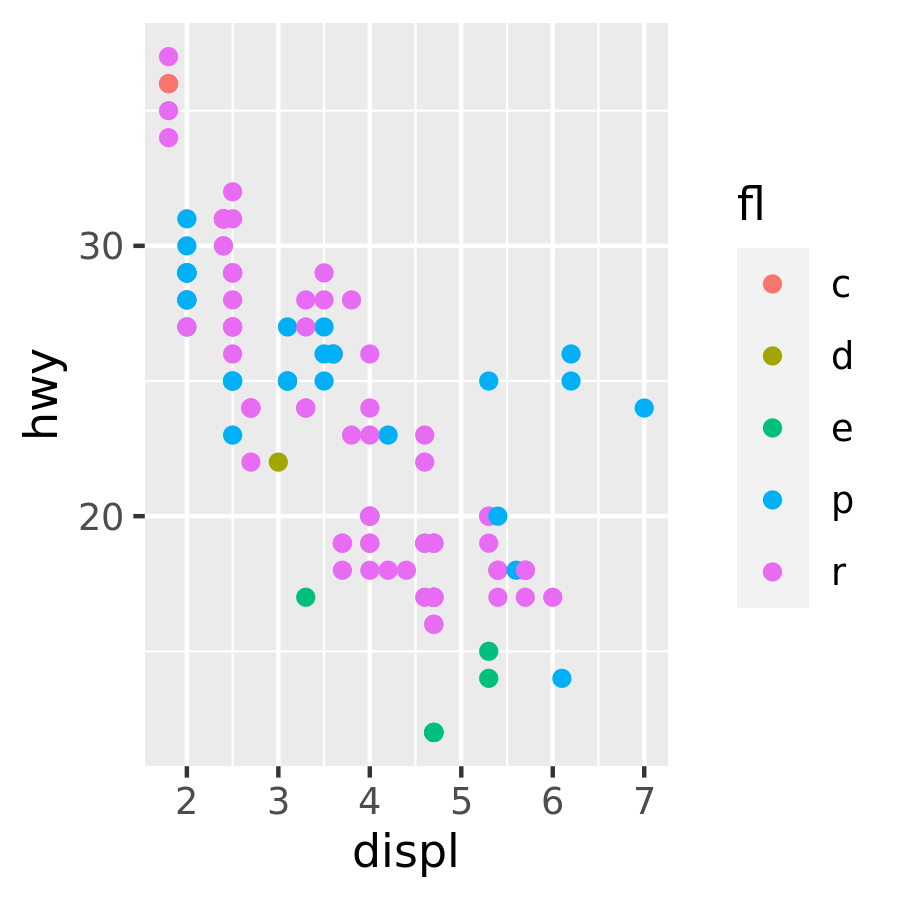
Each plot makes sense on its own, but visual comparison between the two is difficult. The axis limits are different, and because only regular, premium and diesel fuels are represented in the 1998 data the colours are mapped inconsistently.
base_99 +
  scale_x_continuous(limits = c(1, 7)) +
  scale_y_continuous(limits = c(10, 45))

base_08 +
  scale_x_continuous(limits = c(1, 7)) +
  scale_y_continuous(limits = c(10, 45))

In many cases setting the limits for x and y axes would be sufficient to solve the problem, but in this example we still need to ensure that the colour scale is consistent across plots.
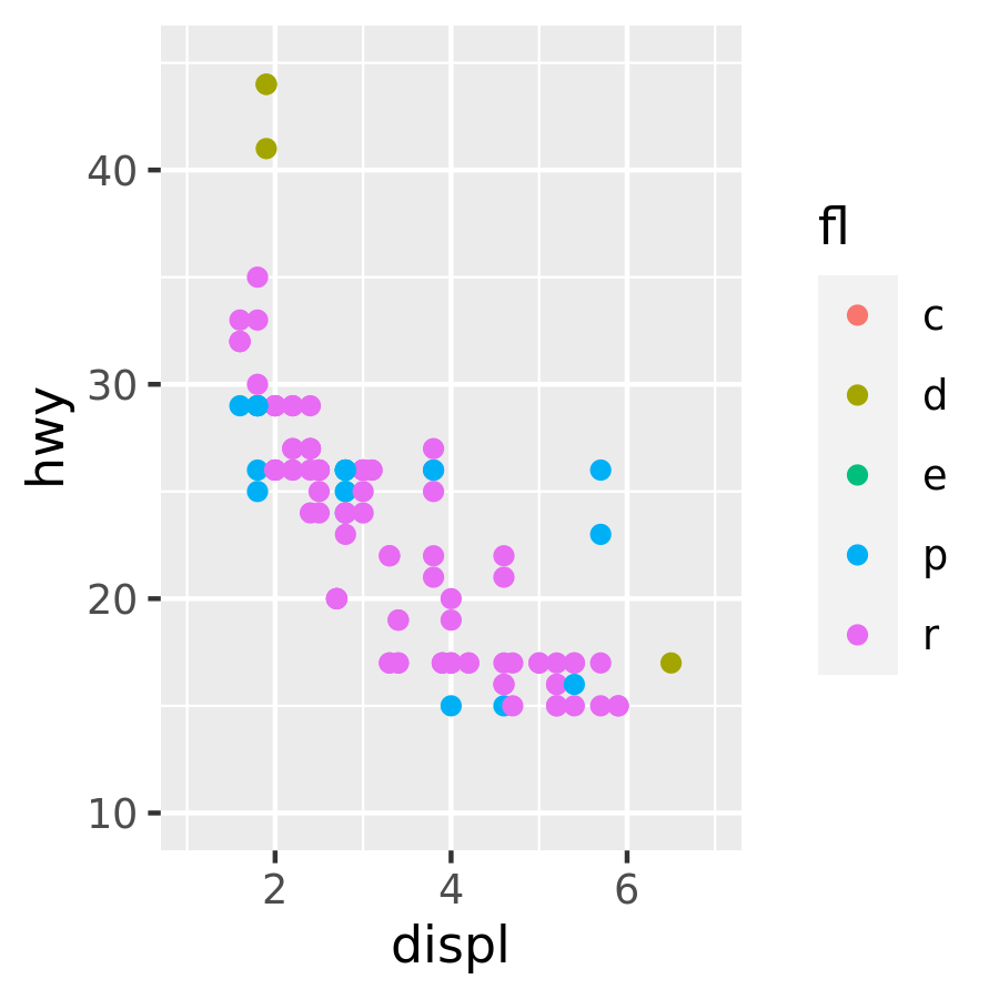
base_99 +
scale_x_continuous(limits = c(1, 7)) +
scale_y_continuous(limits = c(10, 45)) +
scale_color_discrete(limits = c("c", "d", "e", "p", "r"))
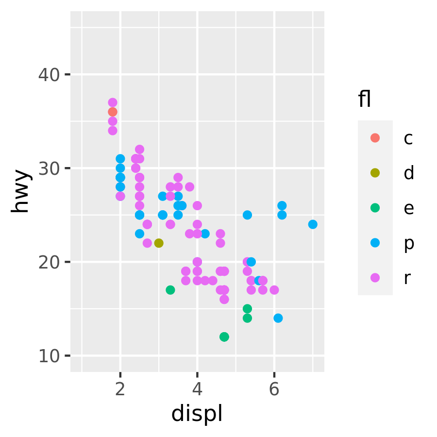
base_08 +
scale_x_continuous(limits = c(1, 7)) +
scale_y_continuous(limits = c(10, 45)) +
scale_color_discrete(limits = c("c", "d", "e", "p", "r"))

Note that because the fuel variable fl is discrete, the limits for the colour aesthetic are a vector of possible values rather than the two end points.
Because modifying scale limits is such a common task, ggplot2 provides some convenience functions to make this easier. For position scales the xlim() and ylim() helper functions inspect their input and then specify the appropriate scale for the x and y axes respectively. The results depend on the type of scale:
xlim(10, 20): a continuous scale from 10 to 20ylim(20, 10): a reversed continuous scale from 20 to 10xlim("a", "b", "c"): a discrete scalexlim(as.Date(c("2008-05-01", "2008-08-01"))): a date scale from May 1 to August 1 2008 (date scales are discussed in Section 9.2.1)
To ensure consistent axis scaling in the previous example, we can use these helper functions:
base_99 + xlim(1, 7) + ylim(10, 45)
base_08 + xlim(1, 7) + ylim(10, 45)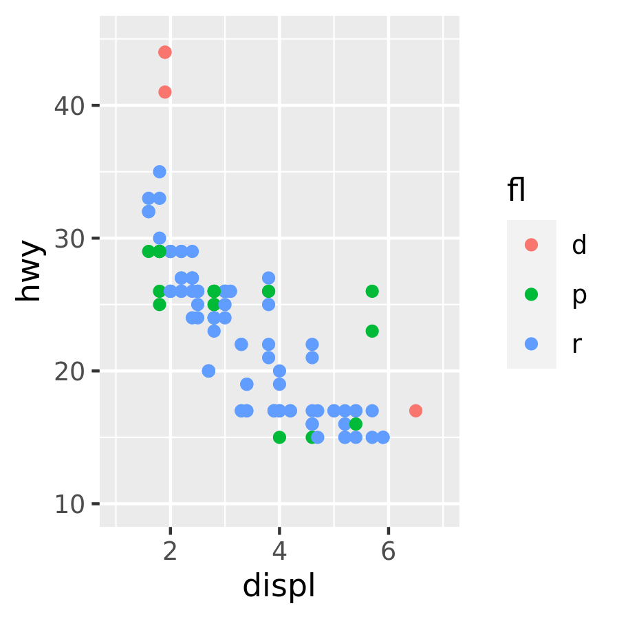

Another option for setting limits is the lims() function which takes name-value pairs as input, where the name specifies the aesthetic and the value specifies the limits:
base_99 + lims(x = c(1, 7), y = c(10, 45), colour = c("c", "d", "e", "p", "r"))
base_08 + lims(x = c(1, 7), y = c(10, 45), colour = c("c", "d", "e", "p", "r"))