6.3 Map projections
At the start of the chapter I drew maps by plotting longitude and latitude on a Cartesian plane, as if geospatial data were no different to other kinds of data one might want to plot. To a first approximation this is okay, but it’s not good enough if you care about accuracy. There are two fundamental problems with the approach.
The first issue is the shape of the planet. The Earth is neither a flat plane, nor indeed is it a perfect sphere. As a consequence, to map a co-ordinate value (longitude and latitude) to a location we need to make assumptions about all kinds of things. How ellipsoidal is the Earth? Where is the centre of the planet? Where is the origin point for longitude and latitude? Where is the sea level? How do the tectonic plates move? All these things are relevant, and depending on what assumptions one makes the same co-ordinate can be mapped to locations that are many meters apart. The set of assumptions about the shape of the Earth is referred to as the geodetic datum and while it might not matter for some data visualisations, for others it is critical. There are several different choices one might consider: if your focus is North America the “North American Datum” (NAD83) is a good choice, whereas if your perspective is global the “World Geodetic System” (WGS84) is probably better.
The second issue is the shape of your map. The Earth is approximately ellipsoidal, but in most instances your spatial data need to be drawn on a two dimensional plane. It is not possible to map the surface of an ellipsoid to a plane without some distortion or cutting, and you will have to make choices about what distortions you are prepared to accept when drawing a map. This is the job of the map projection.
Map projections are often classified in terms of the geometric properties that they preserve, e.g.
Area-preserving projections ensure that regions of equal area on the globe are drawn with equal area on the map.
Shape-preserving (or conformal) projections ensure that the local shape of regions is preserved.
And unfortunately, it’s not possible for any projection to be shape-preserving and area-preserving. This makes it a little beyond the scope of this book to discuss map projections in detail, other than to note that the simple features specification allows you to indicate which map projection you want to use. For more information on map projections, see Geocomputation with R https://geocompr.robinlovelace.net/.22
Taken together, the geodetic datum (e.g, WGS84), the type of map projection (e.g., Mercator) and the parameters of the projection (e.g., location of the origin) specify a coordinate reference system, or CRS, a complete set of assumptions used to translate the latitude and longitude information into a two dimensional map. An sf object often includes a default CRS, as illustrated below:
st_crs(oz_votes)
#> Coordinate Reference System:
#>   User input: EPSG:4283
#>   wkt:
#> GEOGCRS["GDA94",
#>     DATUM["Geocentric Datum of Australia 1994",
#>         ELLIPSOID["GRS 1980",6378137,298.257222101,
#>             LENGTHUNIT["metre",1]]],
#>     PRIMEM["Greenwich",0,
#>         ANGLEUNIT["degree",0.0174532925199433]],
#>     CS[ellipsoidal,2],
#>         AXIS["geodetic latitude (Lat)",north,
#>             ORDER[1],
#>             ANGLEUNIT["degree",0.0174532925199433]],
#>         AXIS["geodetic longitude (Lon)",east,
#>             ORDER[2],
#>             ANGLEUNIT["degree",0.0174532925199433]],
#>     USAGE[
#>         SCOPE["unknown"],
#>         AREA["Australia - GDA"],
#>         BBOX[-60.56,93.41,-8.47,173.35]],
#>     ID["EPSG",4283]]
Most of this output corresponds to a well-known text (WKT) string that unambiguously describes the CRS. This verbose WKT representation is used by sf internally, but there are several ways to provide user input that sf understands. One such method is to provide numeric input in the form of an EPSG code (see http://www.epsg.org/). The default CRS in the oz_votes data corresponds to EPSG code 4283:
st_crs(oz_votes) == st_crs(4283)
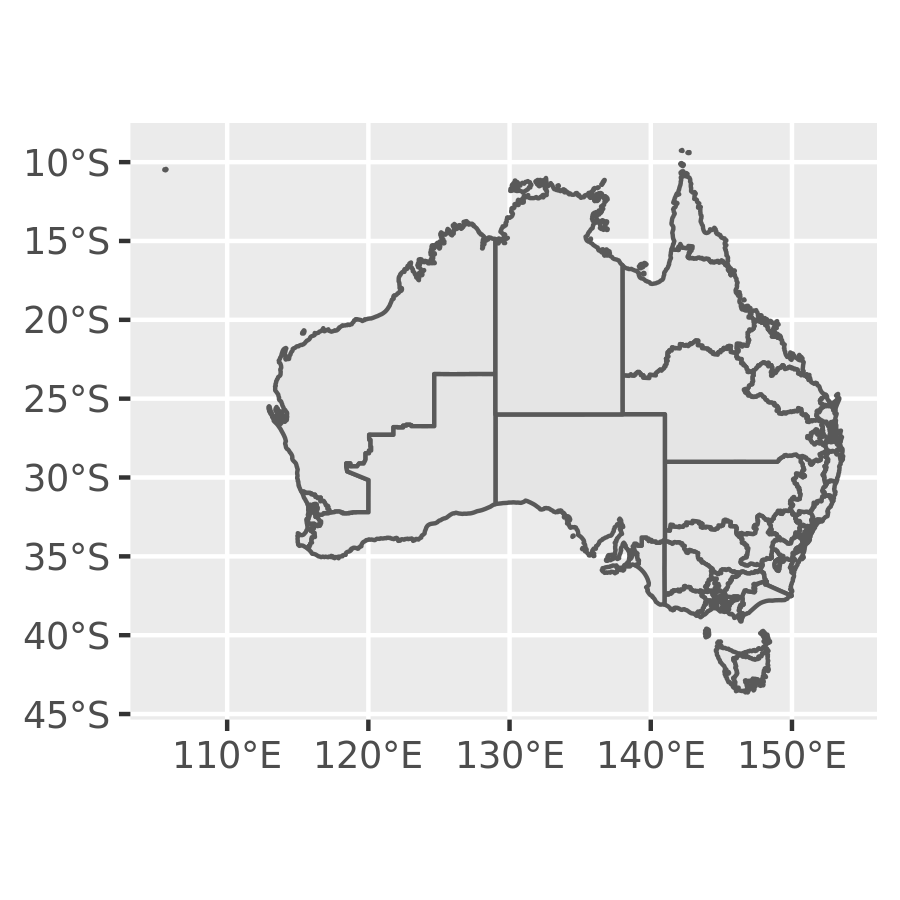
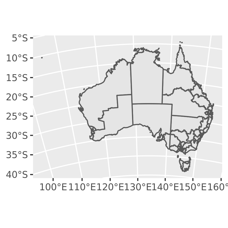
#> [1] TRUEIn ggplot2, the CRS is controlled by coord_sf(), which ensures that every layer in the plot uses the same projection. By default, coord_sf() uses the CRS associated with the geometry column of the data23. Because sf data typically supply a sensible choice of CRS, this process usually unfolds invisibly, requiring no intervention from the user. However, should you need to set the CRS yourself, you can specify the crs parameter by passing valid user input to st_crs(). The example below illustrates how to switch from the default CRS to EPSG code 3112:
ggplot(oz_votes) + geom_sf()
ggplot(oz_votes) + geom_sf() + coord_sf(crs = st_crs(3112))