4.4 Matching aesthetics to graphic objects

A final important issue with collective geoms is how the aesthetics of the individual observations are mapped to the aesthetics of the complete entity. What happens when different aesthetics are mapped to a single geometric element?

In ggplot2, this is handled differently for different collective geoms. Lines and paths operate on a “first value” principle: each segment is defined by two observations, and ggplot2 applies the aesthetic value (e.g., colour) associated with the first observation when drawing the segment. That is, the aesthetic for the first observation is used when drawing the first segment, the second observation is used when drawing the second segment and so on. The aesthetic value for the last observation is not used:

df <- data.frame(x = 1:3, y = 1:3, colour = c(1,3,5))

ggplot(df, aes(x, y, colour = factor(colour))) + 
  geom_line(aes(group = 1), size = 2) +
  geom_point(size = 5)

ggplot(df, aes(x, y, colour = colour)) + 
  geom_line(aes(group = 1), size = 2) +
  geom_point(size = 5)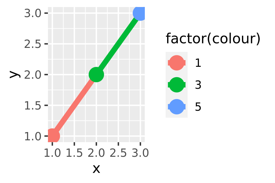

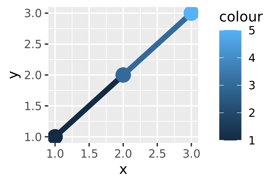
On the left — where colour is discrete — the first point and first line segment are red, the second point and second line segment are green, and the final point (with no corresponding segment) is blue. On the right — where colour is continuous — the same principle is applied to the three different shades of blue. Notice that even though the colour variable is continuous, ggplot2 does not smoothly blend from one aesthetic value to another. If this is the behaviour you want, you can perform the linear interpolation yourself:

xgrid <- with(df, seq(min(x), max(x), length = 50))
interp <- data.frame(
  x = xgrid,
  y = approx(df$x, df$y, xout = xgrid)$y,
  colour = approx(df$x, df$colour, xout = xgrid)$y  
)
ggplot(interp, aes(x, y, colour = colour)) + 
  geom_line(size = 2) +
  geom_point(data = df, size = 5)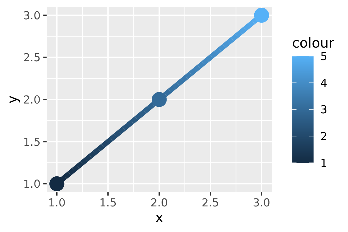

An additional limitation for paths and lines is worth noting: the line type must be constant over each individual line. In R there is no way to draw a line which has varying line type.

What about other collective geoms, such as polygons? Most collective geoms are more complicated than lines and path, and a single geometric object can map onto many observations. In such cases it is not obvious how the aesthetics of individual observations should be combined. For instance, how would you colour a polygon that had a different fill colour for each point on its border? Due to this ambiguity ggplot2 adopts a simple rule: the aesthetics from the individual components are used only if they are all the same. If the aesthetics differ for each component, ggplot2 uses a default value instead.

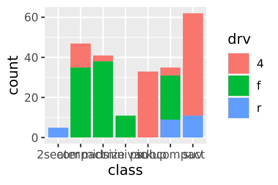
These issues are most relevant when mapping aesthetics to continuous variables. For discrete variables, the default behaviour of ggplot2 is to treat the variable as part of the group aesthetic, as described above. This has the effect of splitting the collective geom into smaller pieces. This works particularly well for bar and area plots, because stacking the individual pieces produces the same shape as the original ungrouped data:

ggplot(mpg, aes(class)) + 
  geom_bar()
ggplot(mpg, aes(class, fill = drv)) + 
  geom_bar()

If you try to map the fill aesthetic to a continuous variable (e.g., hwy) in the same way, it doesn’t work. The default grouping will only be based on class, so each bar is now associated with multiple colours (depending on the value of hwy for the observations in each class). Because a bar can only display one colour, ggplot2 reverts to the default grey in this case. To show multiple colours, we need multiple bars for each class, which we can get by overriding the grouping:

ggplot(mpg, aes(class, fill = hwy)) + 
  geom_bar()
ggplot(mpg, aes(class, fill = hwy, group = hwy)) + 
  geom_bar()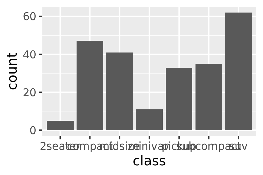

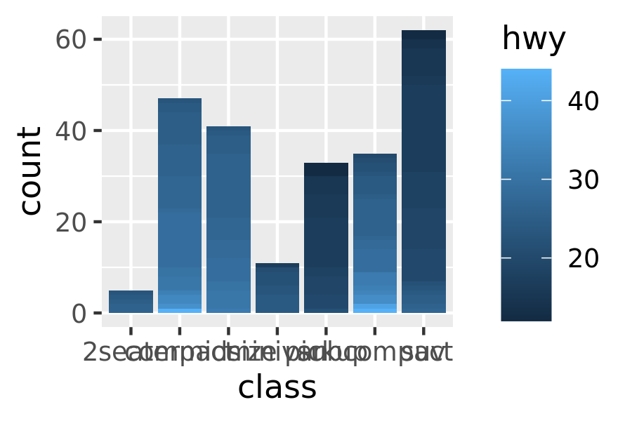
In the plot on the right, the “shaded bars” for each class have been constructed by stacking many distinct bars on top of each other, each filled with a different shade based on the value of hwy. Note that when you do this, the bars are stacked in the order defined by the grouping variable (in this example hwy). If you need fine control over this behaviour, you’ll need to create a factor with levels ordered as needed.