2.8 Output
Most of the time you create a plot object and immediately plot it, but you can also save a plot to a variable and manipulate it:
p <- ggplot(mpg, aes(displ, hwy, colour = factor(cyl))) +
  geom_point()
Once you have a plot object, there are a few things you can do with it:
Render it on screen with
print(). This happens automatically when running interactively, but inside a loop or function, you’ll need toprint()it yourself.print(p)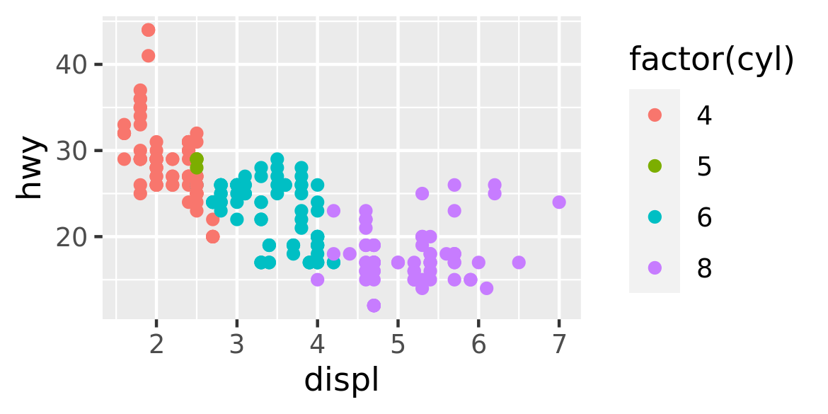
Save it to disk with
ggsave(), described in Section 17.5.# Save png to disk ggsave("plot.png", p, width = 5, height = 5)Briefly describe its structure with
summary().summary(p) #> data: manufacturer, model, displ, year, cyl, trans, drv, cty, hwy, fl, #> class [234x11] #> mapping: x = ~displ, y = ~hwy, colour = ~factor(cyl) #> faceting: <ggproto object: Class FacetNull, Facet, gg> #> compute_layout: function #> draw_back: function #> draw_front: function #> draw_labels: function #> draw_panels: function #> finish_data: function #> init_scales: function #> map_data: function #> params: list #> setup_data: function #> setup_params: function #> shrink: TRUE #> train_scales: function #> vars: function #> super: <ggproto object: Class FacetNull, Facet, gg> #> ----------------------------------- #> geom_point: na.rm = FALSE #> stat_identity: na.rm = FALSE #> position_identitySave a cached copy of it to disk, with
saveRDS(). This saves a complete copy of the plot object, so you can easily re-create it withreadRDS().saveRDS(p, "plot.rds") q <- readRDS("plot.rds")
You’ll learn more about how to manipulate these objects in Chapter 18.