2.5 Faceting

Another technique for displaying additional categorical variables on a plot is faceting. Faceting creates tables of graphics by splitting the data into subsets and displaying the same graph for each subset. You’ll learn more about faceting in Section 16, but it’s such a useful technique that you need to know it right away.

There are two types of faceting: grid and wrapped. Wrapped is the most useful, so we’ll discuss it here, and you can learn about grid faceting later. To facet a plot you simply add a faceting specification with facet_wrap(), which takes the name of a variable preceded by ~.

ggplot(mpg, aes(displ, hwy)) + 
  geom_point() + 
  facet_wrap(~class)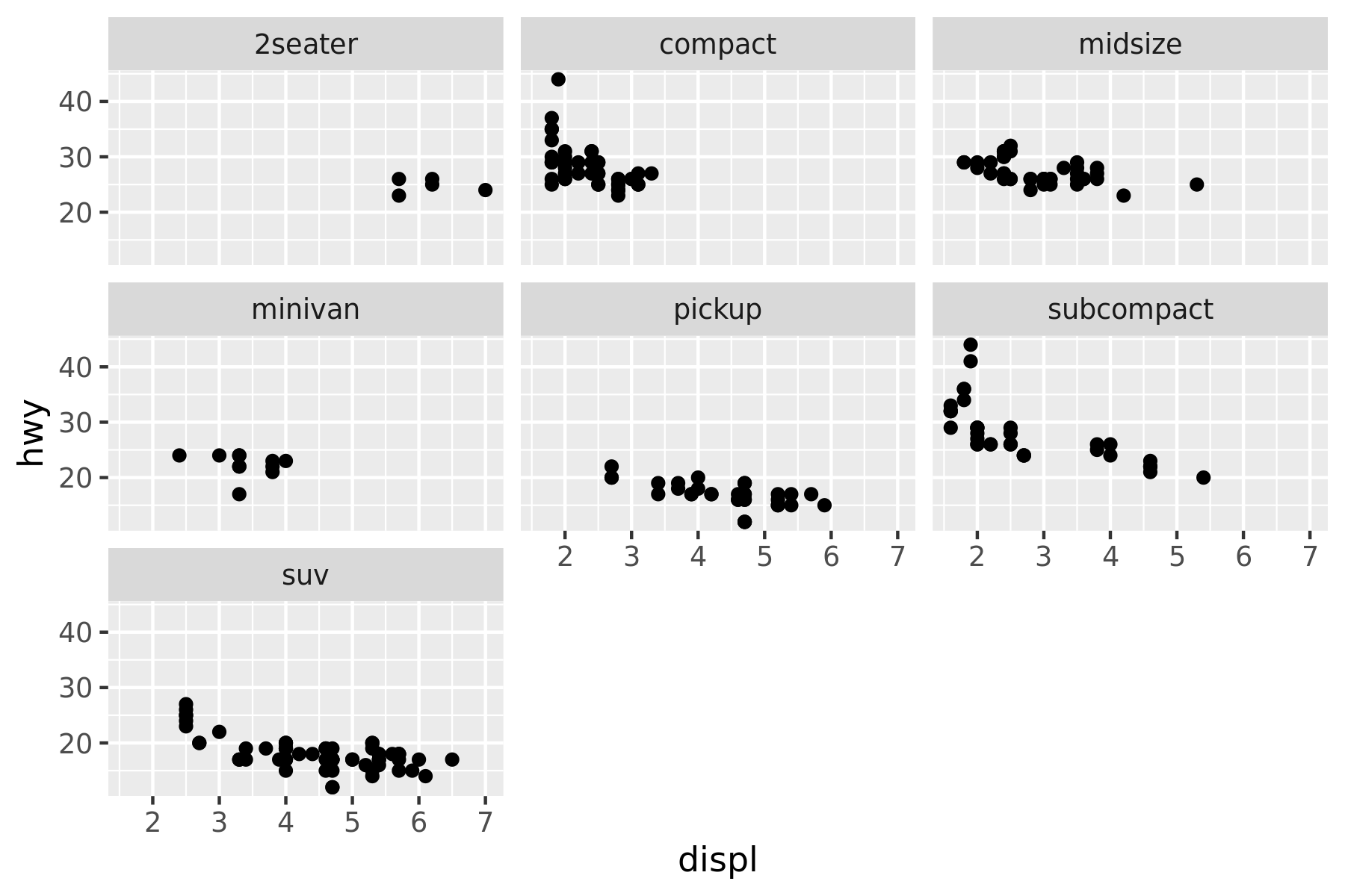

You might wonder when to use faceting and when to use aesthetics. You’ll learn more about the relative advantages and disadvantages of each in Section 16.5.

2.5.1 Exercises

1. What happens if you try to facet by a continuous variable like hwy? What about cyl? What’s the key difference?

2. Use faceting to explore the 3-way relationship between fuel economy, engine size, and number of cylinders. How does faceting by number of cylinders change your assessement of the relationship between engine size and fuel economy?

3. Read the documentation for facet_wrap(). What arguments can you use to control how many rows and columns appear in the output?

4. What does the scales argument to facet_wrap() do? When might you use it?