6.4 Working with sf data
As noted earlier, maps created using geom_sf() and coord_sf() rely heavily on tools
provided by the sf package, and indeed the sf package contains many more useful tools for
manipulating simple features data. In this section I provide an introduction to a few
such tools; more detailed coverage can be found on the sf package website
https://r-spatial.github.io/sf/.
To get started, recall that one advantage to simple features over other representations of spatial data is that geographical units can have complicated structure. A good example of this in the Australian maps data is the electoral district of Eden-Monaro, plotted below:
edenmonaro <- ozmaps::abs_ced %>% filter(NAME == "Eden-Monaro")

p <- ggplot(edenmonaro) + geom_sf()
p + coord_sf(xlim = c(147.75, 150.25), ylim = c(-37.5, -34.5))
p + coord_sf(xlim = c(150, 150.25), ylim = c(-36.3, -36)) 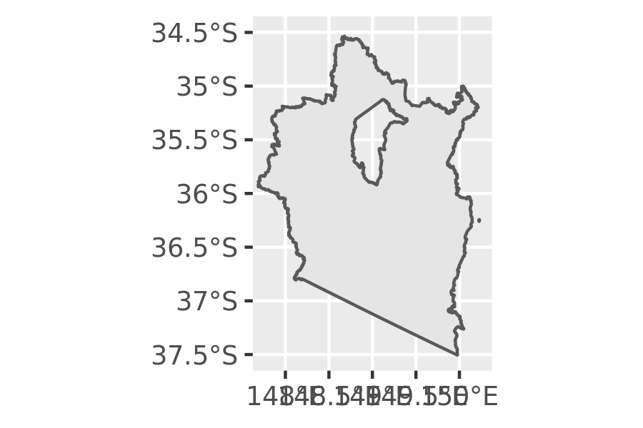
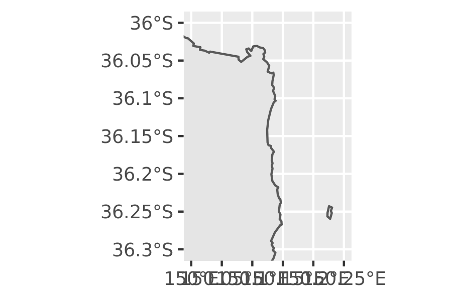
As this illustrates, Eden-Monaro is defined in terms of two distinct polygons, a large one on the Australian mainland and a small island. However, the large region has a hole in the middle (the hole exists because the Australian Capital Territory is a distinct political unit that is wholly contained within Eden-Monaro, and as illustrated above, electoral boundaries in Australia do not cross state lines). In sf terminology this is an example of a MULTIPOLYGON geometry. In this section I’ll talk about the structure of these objects and how to work with them.
First, let’s use dplyr to grab only the geometry object:
edenmonaro <- edenmonaro %>% pull(geometry)The metadata for the edenmonaro object can accessed using helper functions. For example, st_geometry_type() extracts the geometry type (e.g., MULTIPOLYGON), st_dimension() extracts the number of dimensions (2 for XY data, 3 for XYZ), st_bbox() extracts the bounding box as a numeric vector, and st_crs() extracts the CRS as a list with two components, one for the EPSG code and the other for the proj4string. For example:
st_bbox(edenmonaro)
#>  xmin  ymin  xmax  ymax
#> 147.7 -37.5 150.2 -34.5
Normally when we print the edenmonaro object the output would display all the additional information (dimension, bounding box, geodetic datum etc) but for the remainder of this section I will show only the relevant lines of the output. In this case edenmonaro is defined by a MULTIPOLYGON geometry containing one feature:
edenmonaro
#> Geometry set for 1 feature
#> geometry type:  MULTIPOLYGON
#> MULTIPOLYGON (((150 -36.2, 150 -36.2, 150 -36.3...
However, we can “cast” the MULTIPOLYGON into the two distinct POLYGON geometries from which it is constructed using st_cast():
st_cast(edenmonaro, "POLYGON")
#> Geometry set for 2 features
#> geometry type:  POLYGON
#> POLYGON ((150 -36.2, 150 -36.2, 150 -36.3, 150 ...
#> POLYGON ((148 -36.7, 148 -36.7, 148 -36.7, 148 ...
To illustrate when this might be useful, consider the Dawson electorate, which consists of 69 islands in addition to a coastal region on the Australian mainland.
dawson <- ozmaps::abs_ced %>%
  filter(NAME == "Dawson") %>%
  pull(geometry)
dawson
#> Geometry set for 1 feature
#> geometry type:  MULTIPOLYGON
#> MULTIPOLYGON (((148 -19.9, 148 -19.8, 148 -19.8...

ggplot(dawson) +
  geom_sf() +
  coord_sf()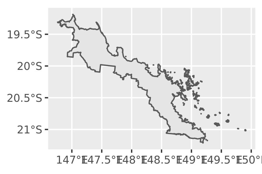
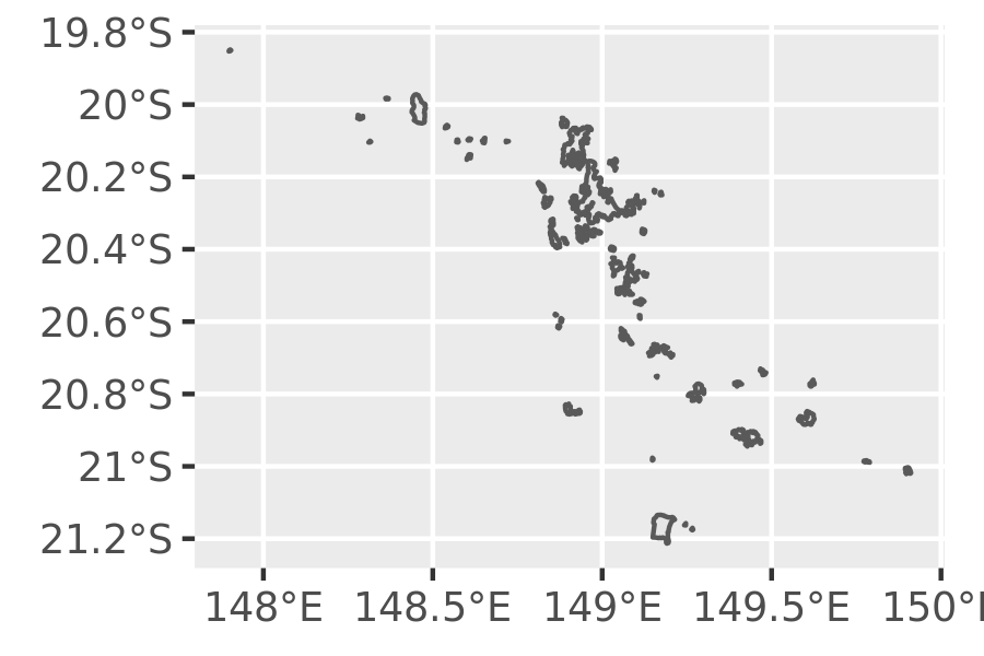
Suppose, however, our interest is only in mapping the islands. If so, we can first use the st_cast() function to break the Dawson electorate into the constituent polygons. After doing so, we can use st_area() to calculate the area of each polygon and which.max() to find the polygon with maximum area:
dawson <- st_cast(dawson, "POLYGON")
which.max(st_area(dawson))
#> [1] 69
The large mainland region corresponds to the 69th polygon within Dawson. Armed with this knowledge, we can draw a map showing only the islands:
ggplot(dawson[-69]) +
  geom_sf() +
  coord_sf()