21.4 Part 3: A geom

In many cases a Stat-centred approach is sufficient, for example, many of the graphic primitives provided by the ggforce package are Stats. But we need to go further with the spring geom because the tension and diameter aesthetics need specified in units that are unrelated to the coordinate system. Consequently, we’ll rewrite our geom to be a proper Geom extension.

21.4.1 Geom extensions

As discussed in Section 20, there are many similarities between Stat and Geom extensions. The biggest difference is that Stat extensions return a modified version of the input data, whereas Geom extensions return graphical objects (technically, grid grobs; more on that later).

Since our geom is a special type of a path, we can get pretty far by simply extending GeomPath and modifying the data before it is rendered:

GeomSpring <- ggproto("GeomSpring", GeomPath,
  ...,
  setup_data = function(data, params) {
    cols_to_keep <- setdiff(names(data), c("x", "y", "xend", "yend"))
    springs <- lapply(seq_len(nrow(data)), function(i) {
      spring_path <- create_spring(
        data$x[i], data$y[i], data$xend[i], data$yend[i], 
        diameter = data$diameter[i],
        tension = data$tension[i], 
        n = params$n
      )
      spring_path <- cbind(spring_path, unclass(data[i, cols_to_keep]))
      spring_path$group <- i
      spring_path
    })
    do.call(rbind, springs)
  },
  ...
)

Here we override the the setup_data() method, applying create_spring() to each row. This is simple, but isn’t really an improvement over our StatSpring approach because setup_data() is called before the default and set aesthetics are added to the data, so it will only work if everything is defined within aes().

To make things better, we’ll need to move our data manipulation into the draw_*() methods. Fortunately, we can re-use the GeomPath implementation so we don’t yet have to learn about exactly what type of output we need to produce:

GeomSpring <- ggproto("GeomSpring", Geom,
  setup_data = function(data, params) {
    if (is.null(data$group)) {
      data$group <- seq_len(nrow(data))
    }
    if (anyDuplicated(data$group)) {
      data$group <- paste(data$group, seq_len(nrow(data)), sep = "-")
    }
    data
  },
  draw_panel = function(data, panel_params, coord, n = 50, arrow = NULL,
                        lineend = "butt", linejoin = "round", linemitre = 10,
                        na.rm = FALSE) {
    cols_to_keep <- setdiff(names(data), c("x", "y", "xend", "yend"))
    springs <- lapply(seq_len(nrow(data)), function(i) {
      spring_path <- create_spring(data$x[i], data$y[i], data$xend[i], 
                                   data$yend[i], data$diameter[i],
                                   data$tension[i], n)
      cbind(spring_path, unclass(data[i, cols_to_keep]))
    })
    springs <- do.call(rbind, springs)
    GeomPath$draw_panel(
      data = springs, 
      panel_params = panel_params, 
      coord = coord, 
      arrow = arrow, 
      lineend = lineend, 
      linejoin = linejoin, 
      linemitre = linemitre, 
      na.rm = na.rm
    )
  },
  required_aes = c("x", "y", "xend", "yend"),
  default_aes = aes(
    colour = "black", 
    size = 0.5, 
    linetype = 1L, 
    alpha = NA, 
    diameter = 1, 
    tension = 0.75
  )
)

Developers used to object-oriented design may frown upon this design where we call the method of another kindred object directly (GeomPath$draw_panel()), but since Geom objects are stateless this is as safe as subclassing GeomPath and calling the parent method. You can see this approach all over the place in the ggplot2 source code.

If you compare this code to our StatSpring implementation in the last chapter you can see that the compute_panel() and draw_panel() methods are quite similar with the main difference being that we pass on the computed spring coordinates to GeomPath$draw_panel() in the latter method. Our setup_data() method has been greatly simplified because we now relies on the default_aes functionality in Geom to fill out non-mapped aesthetics.

Creating the geom_spring() constructor is almost similar, except that we now uses the identity stat instead of our spring stat and uses the new GeomSpring instead of GeomPath.

geom_spring <- function(mapping = NULL, data = NULL, stat = "identity", 
                        position = "identity", ..., n = 50, arrow = NULL, 
                        lineend = "butt", linejoin = "round", na.rm = FALSE,
                        show.legend = NA, inherit.aes = TRUE) {
  layer(
    data = data, 
    mapping = mapping, 
    stat = stat, 
    geom = GeomSpring, 
    position = position, 
    show.legend = show.legend, 
    inherit.aes = inherit.aes, 
    params = list(
      n = n, 
      arrow = arrow, 
      lineend = lineend, 
      linejoin = linejoin, 
      na.rm = na.rm, 
      ...
    )
  )
}

Without much additional work we now have a proper geom with working default aesthetics and the possibility of setting aesthetics as parameters.

ggplot(some_data, aes(x, y, xend = xend, yend = yend)) + 
  geom_spring(diameter = 0.5)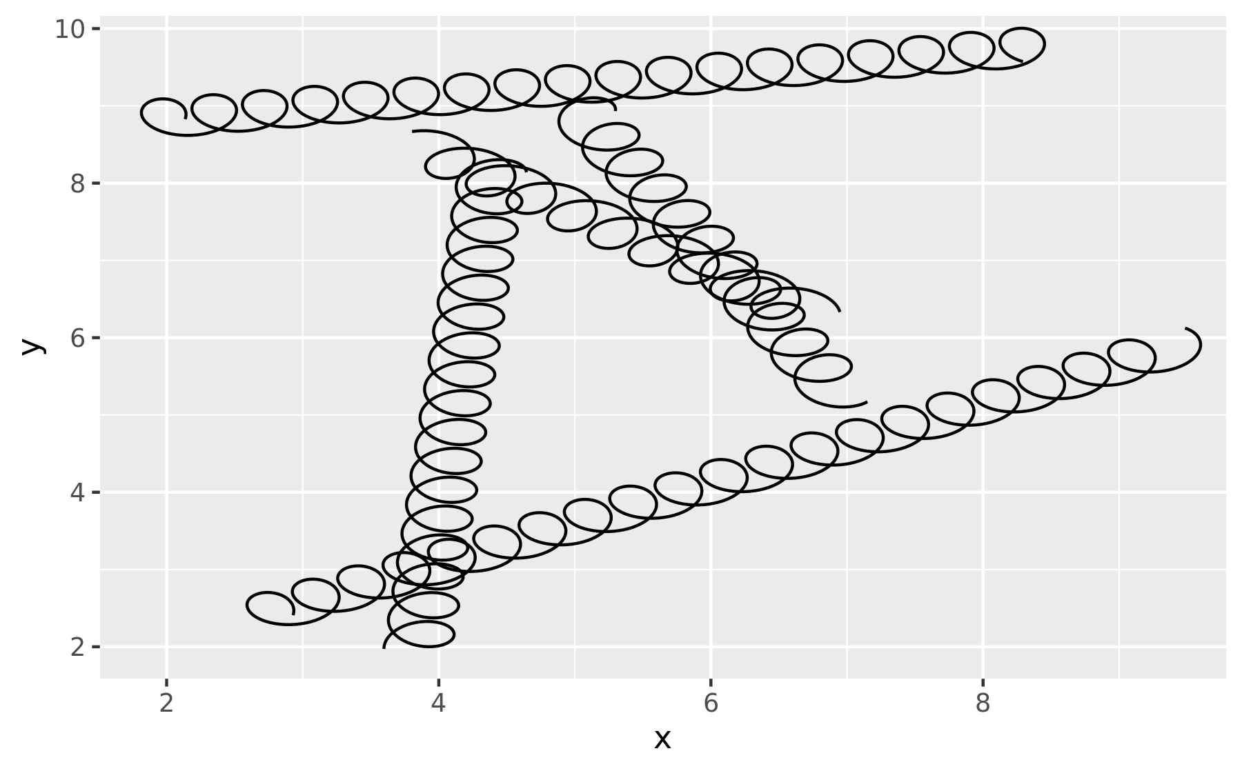

This is basically as far as we can get without learning about grid grobs, the underlying object that actually does the drawing. Creating grid grobs is an advanced technique, needed by relatively few geoms. But creating a grid grob gives you the power to use absolute units (e.g. 1cm) and to adjust the display of the geom based on the size of the output device.

21.4.2 Post-Mortem

In this section we finally created a full Geom extension that behaves as you’d expect. This is often, but not always, the natural conclusion to the development of new layer. The chief advantage of the Stat approach is that you can use the same stat with multiple geoms. The final choice is ultimately up to you and should be guided by how you envision the layer to be used.

We haven’t talked about what goes on inside the draw_*() methods yet. Often it is enough to use a method from existing geom. For example, even the relatively component GeomBoxplot just uses the draw methods from GeomPoint(), GeomSegment and GeomCrossbar. But if you need to go deeper, you’ll need to learn a little about grid