21.5 Part 4: A grid grob
In the last section we exhausted our options for our spring geom safe for delving into the development of a new grid grob. grid is the underlying graphic system that ggplot2 builds upon and while much can be achieved by ignoring grid entirely, there are situations where it is impossible to achieve what you want without going down to the grid level. There are especially two situations that warrant the need for using grid directly when developing ggplot2 extensions:
You need to create graphical objects that are positioned correctly on the coordinate system, but where some part of their appearance has a fixed absolute size. In our case this would be the spring correctly going between two points in the plot, but the diameter being defined in cm instead of relative to the coordinate system.
You need graphical objects that are updated during resizing. This could e.g. be the position of labels such as in the ggrepel package or the
geom_mark_*()geoms in ggforce.
Before we begin developing the new version of our geom it will be good to have at least a cursory understanding of the key concepts in grid:
21.5.1 Grid in 5 minutes
There are two drawing systems included in base R: base graphics and grid. Base graphics has an imperative “pen-on-paper” model: every function immediately draws something on the graphics device. Grid takes a more declarative approach where you build up a nested description of the graphic as an object, which is later rendered (much like ggplot2). This gives us an object that exists independently of the graphic device and can be passed around, analysed, and modified. Importantly, parts of the object can refer to other parts, so that you can say (e.g.) make this rectangle as wide as that string of text.
The next few sections will give you the absolute minimum vocabulary to understand ggplot2’s use of grid: grobs, viewports, and units. To get a sufficient understanding of grid to create your own geoms, we highly recommend Paul Murrell.49
21.5.1.1 Grobs
Grobs (graphic objects) are the atomic representations of graphical elements in grid, and include types like points, lines, rectangles, and text.
All grid objects are vectorised, so that (e.g.) a point grob can represent multiple points.
As well as simple geometric primitive, grid also comes the means to combine multiple grobs into a complex objects called gTree()s.
You can create a new grob new grob classes with the grob() or gTree() constructors, and then give it special behaviour by override the makeContext() and makeContent() S3 generics:
makeContext()is called when the parent grob is rendered and allows you to control the viewport of the grob (see below).makeContent()is called everytime the drawing region is resized and allows you to customise the look based on the size or other aspect.
21.5.1.2 Viewports
grid viewports define rectangular plotting regions. Each viewport defines a coordinate system for position grobs, and optionally, a tabular grid that child viewports can occupy. A grob can have its own viewport or inherit the viewport of its parent. While we won’t need to consider viewports for our spring grob, they’re an important concept that powers much of the high-level layout of ggplot2 graphics.
21.5.1.3 Units
grid units provide a flexible way of specifying positions (e.g. x and y) and dimensions (e.g. length and width) of grobs and viewports.
There are three types of unit:
- Absolute units (e.g. centimeters, inches, and points).
- Relative units (e.g. npc which scales the viewport size between 0 and 1).
- Units based on other grobs (e.g. grobwidth).
units support arithmetic operations and are only resolved at draw time so it is possible to combine different types of units.
For example unit(0.5, "npc") + unit(1, "cm") defines a point one centimeter to the right of the center of the current viewport.
21.5.1.4 Example
Given this very cursory introduction, let’s now look at an example grob. The code below will create a grob that appears as a square if bigger than 5 cm and a circle if smaller::
library(grid)

surpriseGrob <- function(x, y, size,
                         default.units = "npc",
                         name = NULL,
                         gp = gpar(),
                         vp = NULL) {
  # Check if input needs to be converted to units
  if (!is.unit(x)) {
    x <- unit(x, default.units)
  }
  if (!is.unit(y)) {
    y <- unit(y, default.units)
  }
  if (!is.unit(size)) {
    size <- unit(size, default.units)
  }
  # Construct our surprise grob subclass as a gTree
  gTree(
    x = x,
    y = y,
    size = size,
    name = name,
    gp = gp,
    vp = vp,
    cl = "surprise"
  )
}
makeContent.surprise <- function(x) {
  x_pos <- x$x
  y_pos <- x$y
  size <- convertWidth(x$size, unitTo = "cm", valueOnly = TRUE)

  # Figure out if the given sizes are bigger or smaller than 5 cm
  circles <- size < 5

  # Create a circle grob for the small ones
  if (any(circles)) {
    circle_grob <- circleGrob(
      x = x_pos[circles],
      y = y_pos[circles],
      r = unit(size[circles] / 2, "cm")
    )
  } else {
    circle_grob <- nullGrob()
  }

  # Create a rect grob for the large ones
  if (any(!circles)) {
    square_grob <- rectGrob(
      x = x_pos[!circles],
      y = y_pos[!circles],
      width = unit(size[!circles], "cm"),
      height = unit(size[!circles], "cm")
    )
  } else {
    square_grob <- nullGrob()
  }

  # Add the circle and rect grob as childrens of our input grob
  setChildren(x, gList(circle_grob, square_grob))
}

# Create an instance of our surprise grob defining to object with different
# sizes
gr <- surpriseGrob(x = c(0.25, 0.75), y = c(0.5, 0.5), size = c(0.1, 0.4))

# Draw it
grid.newpage()
grid.draw(gr)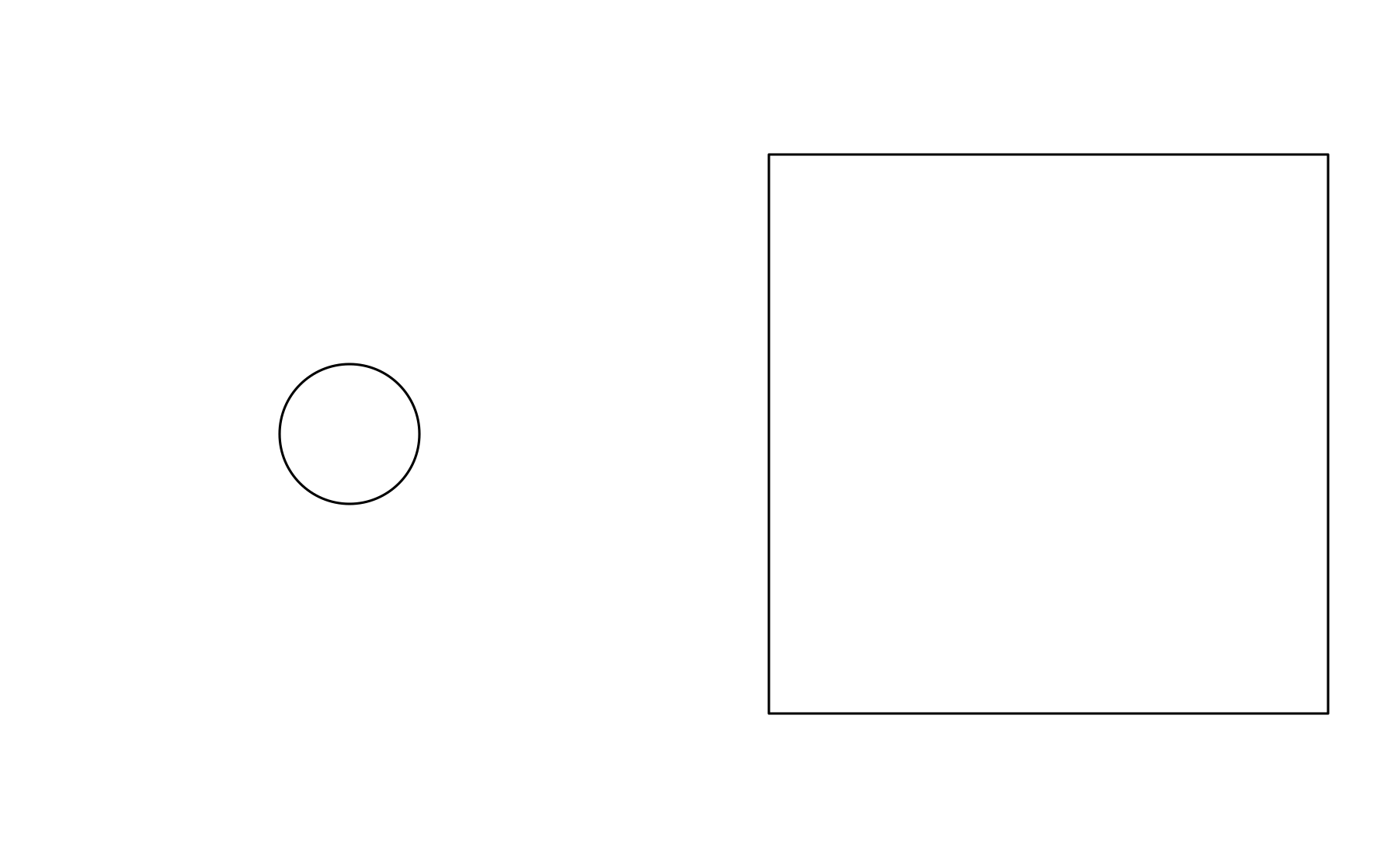
If you run the code above interactively and resize the plotting window you can see that the two objects will change form based on the size of the plotting window. This is a useless example, of course, but hopefully you can see how this technique can be used to do real work.
21.5.2 The springGrob
With our new knowledge of the grid system we can now see how we might construct a spring grob that have an absolute diameter.
If we wait with the expansion to the spring path until the makeContent() function, and calculate it based on coordinates in absolute units we can make sure that the diameter stays constant during resizing of the plot.
With that in mind, we can create our constructor.
We model the arguments after segmentsGrob() since we are basically creating modified segments:
springGrob <- function(x0 = unit(0, "npc"), y0 = unit(0, "npc"),
                       x1 = unit(1, "npc"), y1 = unit(1, "npc"),
                       diameter = unit(0.1, "npc"), tension = 0.75,
                       n = 50, default.units = "npc", name = NULL,
                       gp = gpar(), vp = NULL) {
  if (!is.unit(x0)) x0 <- unit(x0, default.units)
  if (!is.unit(x1)) x1 <- unit(x1, default.units)
  if (!is.unit(y0)) y0 <- unit(y0, default.units)
  if (!is.unit(y1)) y1 <- unit(y1, default.units)
  if (!is.unit(diameter)) diameter <- unit(diameter, default.units)
  gTree(x0 = x0, y0 = y0, x1 = x1, y1 = y1, diameter = diameter,
       tension = tension, n = n, name = name, gp = gp, vp = vp,
       cl = "spring")
}
We see that once again our constructor is a very thin wrapper around the gTree() constructor, simply ensuring that arguments are converted to units if they are not already.
We now need to create the makeContent() method that creates the actual spring coordinates.
makeContent.spring <- function(x) {
  x0 <- convertX(x$x0, "mm", valueOnly = TRUE)
  x1 <- convertX(x$x1, "mm", valueOnly = TRUE)
  y0 <- convertY(x$y0, "mm", valueOnly = TRUE)
  y1 <- convertY(x$y1, "mm", valueOnly = TRUE)
  diameter <- convertWidth(x$diameter, "mm", valueOnly = TRUE)
  tension <- x$tension
  n <- x$n
  springs <- lapply(seq_along(x0), function(i) {
    cbind(
      create_spring(x0[i], y0[i], x1[i], y1[i], diameter[i], tension[i], n),
      id = i
    )
  })
  springs <- do.call(rbind, springs)
  spring_paths <- polylineGrob(springs$x, springs$y, springs$id,
                               default.units = "mm", gp = x$gp)
  setChildren(x, gList(spring_paths))
}
There is not anything fancy going on here.
We grabs the coordinates and diameter settings from the gTree and converts them all to millimeters.
As we now have everything in absolute units we calculate the spring paths using our trusted create_spring() function and puts the returned coordinates in a polyline grob.
Before we use this in a geom let us test it out:
springs <- springGrob(
  x0 = c(0, 0),
  y0 = c(0, 0.5),
  x1 = c(1, 1),
  y1 = c(1, 0.5),
  diameter = unit(c(1, 3), "cm"),
  tension = c(0.2, 0.7)
)
grid.newpage()
grid.draw(springs)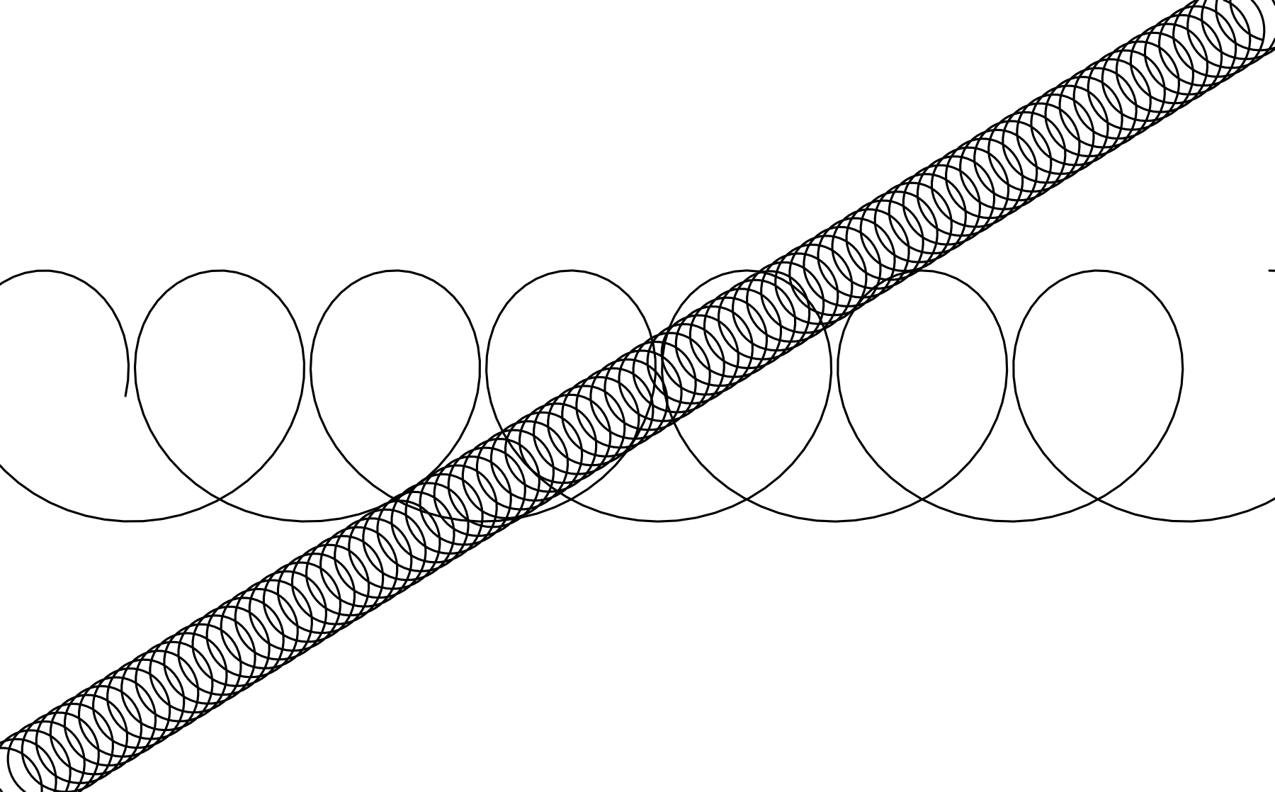
It appears to work and we can now design our new (and final) geom.
21.5.3 The last GeomSpring
GeomSpring <- ggproto("GeomSpring", Geom,
  setup_params = function(data, params) {
    if (is.null(params$n)) {
      params$n <- 50
    } else if (params$n <= 0) {
      rlang::abort("Springs must be defined with `n` greater than 0")
    }
    params
  },
  draw_panel = function(data, panel_params, coord, n = 50, lineend = "butt",
                        na.rm = FALSE) {
    data <- remove_missing(data, na.rm = na.rm,
      c("x", "y", "xend", "yend", "linetype", "size"),
      name = "geom_spring")
    if (is.null(data) || nrow(data) == 0) return(zeroGrob())
    if (!coord$is_linear()) {
      rlang::warn("spring geom only works correctly on linear coordinate systems")
    }
    coord <- coord$transform(data, panel_params)
    return(springGrob(coord$x, coord$y, coord$xend, coord$yend,
      default.units = "native", diameter = unit(coord$diameter, "cm"),
      tension = coord$tension, n = n,
      gp = gpar(
        col = alpha(coord$colour, coord$alpha),
        lwd = coord$size * .pt,
        lty = coord$linetype,
        lineend = lineend
      )
    ))
  },
  required_aes = c("x", "y", "xend", "yend"),
  default_aes = aes(
    colour = "black",
    size = 0.5,
    linetype = 1L,
    alpha = NA,
    diameter = 0.35,
    tension = 0.75
  )
)
geom_spring <- function(mapping = NULL, data = NULL, stat = "identity",
                        position = "identity", ..., n = 50, lineend = "butt",
                        na.rm = FALSE, show.legend = NA, inherit.aes = TRUE) {
  layer(
    data = data,
    mapping = mapping,
    stat = stat,
    geom = GeomSpring,
    position = position,
    show.legend = show.legend,
    inherit.aes = inherit.aes,
    params = list(
      n = n,
      lineend = lineend,
      na.rm = na.rm,
      ...
    )
  )
}
The main differences from our last GeomSpring implementation is that we no longer care about a group column because each spring is defined in one line, and then of course the draw_panel() method.
Since we are no longer passing on the call to another geoms draw_panel() method we have additional obligations in that call.
If the coordinate system is no linear (e.g. coord_polar()) we emit a warning because our spring will not be adapted to that coordinate system.
We then use the coordinate system to rescale our positional aesthetics with the transform() method.
This will remap all positional aesthetics to lie between 0 and 1, with 0 being the lowest value visible in our viewport (scale expansions included) and 1 being the highest.
With this remapping the coordinates are ready to be passed into a grob as "npc" units.
By definition we understands the provided diameter as been given in centimeters.
With all the values properly converted we call the springGrob() constructor and return the resulting grob.
One thing we haven’t touched upon is the gpar() call inside the springGrob() construction.
grid operates with a short list of very well-defined visual characteristics for grobs that are given by the gp argument in the constructor.
This takes a gpar object that holds information such as colour of the stroke and fill, linetype, font, size, etc.
Not all grobs care about all entries in gpar() and since we are constructing a line we only care about the gpar entries that the pathGrob understands, namely: col (stroke colour), lwd (line width), lty (line type), lineend (the terminator shape of the line).
ggplot(some_data) +
  geom_spring(aes(
    x = x,
    y = y,
    xend = xend,
    yend = yend,
    diameter = diameter,
    tension = tension
  ))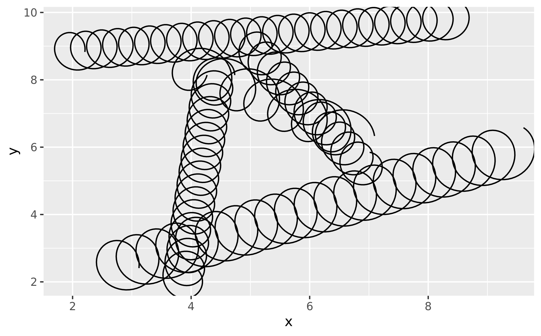
As can be seen in the example above we now have springs that do not shear with the aspect ratio of the plot and thus looks conform at every angle and aspect ratio. Further, resizing the plot will result in recalculations of the correct path so that it will continues to look as it should.
21.5.4 Post-Mortem
We have finally arrived at the spring geom we set out to make.
The diameter of the spring behaves in the same way as a line width in that it remains fixed when resizing and/or changing the aspect ratio of the plot.
There are still improvements we could (and perhaps, should) do to our geom.
Most notably our create_spring() function remains un-vectorised and needs to be called for each spring separately.
Correctly vectorizing this function will allow for considerable speed-up when rendering many springs (if that was ever a need).
We will leave this as an exercise for the reader.
While the geom is now done, we still a have a little work to do. We need to create a diameter scale and provide legend keys that can correctly communicate diameter and tension. This will be the topic of the final section.
R Graphics, Second (Chapman & Hall/CRC, 2011), https://www.stat.auckland.ac.nz/~paul/RG2e/.↩︎