21.6 Part 5: Scales
Now that we have our final geom, there’s still a bit of work to do before we are done. This is because we have defined a couple of new aesthetics in the process and we would like users to be able to scale them. There’s nothing wrong with defining new aesthetics without providing a scale — that simply means that the mapped values are passed through unchanged — but if we want users to have some control as well as the possibility of a legend we will need to provide scales for the aesthetics. This will be the goal of this final section.
21.6.1 Scaling
Thankfully, compared to grid, creating new scales is not a huge undertaking.
It basically surmounts to creating a function with the correct name that outputs a Scale object.
In the code below you can see how this is done for the tension aesthetic:
scale_tension_continuous <- function(..., range = c(0.1, 1)) {
  continuous_scale(
    aesthetics = "tension",
    scale_name = "tension_c",
    palette = scales::rescale_pal(range),
    ...
  )
}
Most scale functions are simply wrappers around calls to one of the scale constructors (continuous_scale(), discrete_scale(), and binned_scale()).
Most importantly it names the aesthetic(s) this scale relates to and provides a palette function which transforms the input domain to the output range.
All the remaining well-known arguments from scale functions such as name, breaks, limits, etc. are carried through with the ....
For cases such as these where only a single scale is relevant for an aesthetic you’ll often create a short-named version as well.
We’ll also add a discrete scale to catch if this aesthetic is erroneously being used with discrete data:
scale_tension <- scale_tension_continuous

scale_tension_discrete <- function(...) {
  rlang::abort("Tension cannot be used with discrete data")
}
The reason why we need scale_tension_continuous() when we also have scale_tension() is that the default scale for aesthetics is looked up by searching for a function called scale_<aesthetic-name>_<data-type>.
While we are at it we’ll create a scale for the diameter as well:
scale_diameter_continuous <- function(..., range = c(0.25, 0.7), unit = "cm") {
  range <- grid::convertWidth(unit(range, unit), "cm", valueOnly = TRUE)
  continuous_scale(
    aesthetics = "diameter",
    scale_name = "diameter_c",
    palette = scales::rescale_pal(range),
    ...
  )
}
scale_diameter <- scale_diameter_continuous
scale_tension_discrete <- function(...) {
  rlang::abort("Diameter cannot be used with discrete data")
}
The only change we made from the tension scales is that we allow the user to define which unit the diameter range should be measured in.
Since the geom expects centimeters we will convert the range to that before passing it into the scale constructor.
In that way the user is free to use whatever absolute unit feels natural to them.
With our scales defined let us have a look:
ggplot(some_data) +
  geom_spring(aes(x = x, y = y, xend = xend, yend = yend, tension = tension,
                  diameter = diameter)) +
  scale_tension(range = c(0.1, 5))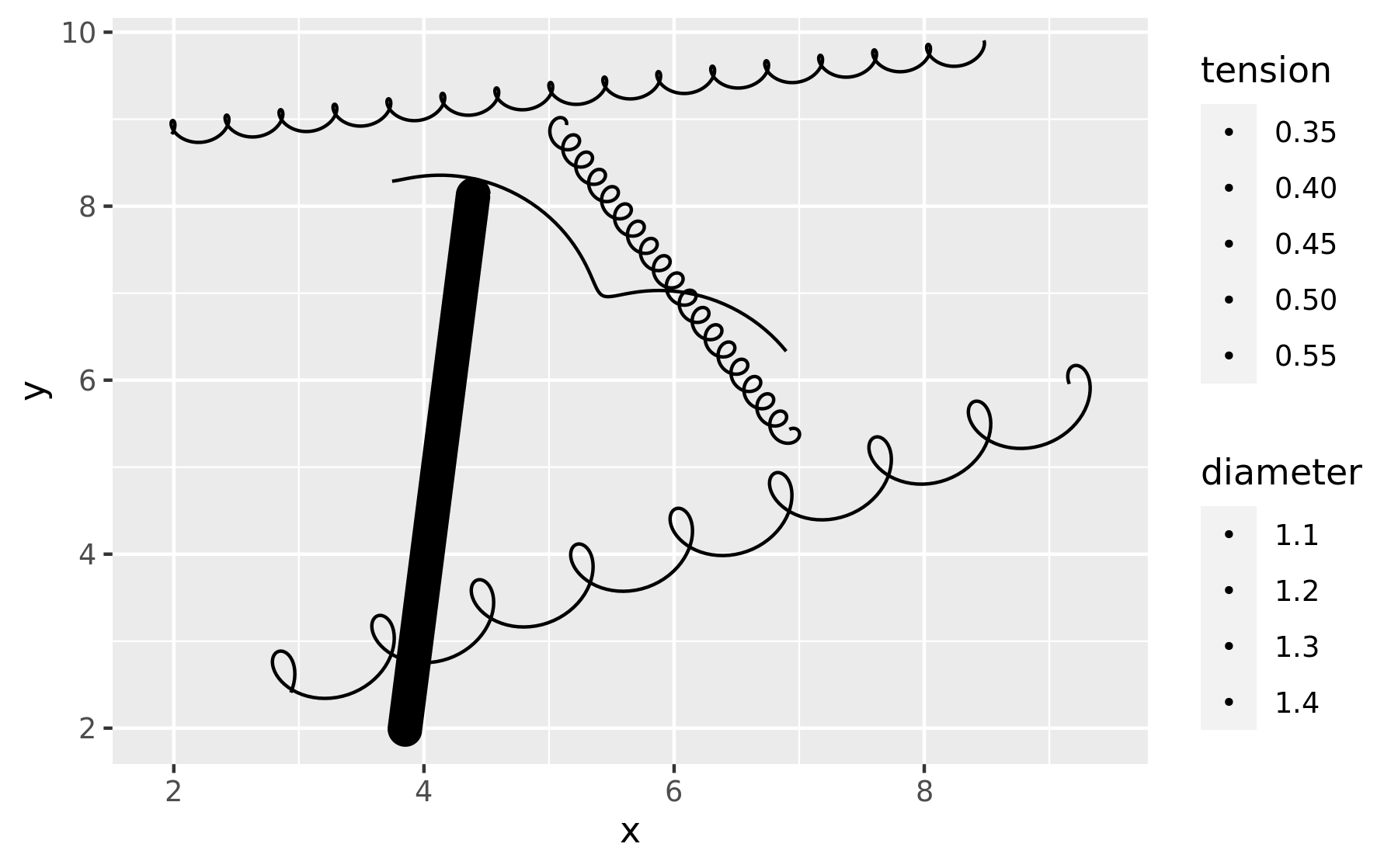
The code above shows us that both the default scale (we didn’t add an explicit scale for diameter) and the custom scales (scale_tension()) work.
It also tells us that our job is not done, because the legend is pretty uninformative.
That is because our geom uses the default legend key constructor which is draw_key_point().
This key constructor doesn’t know what to do about our new aesthetics and ignores it completely.
21.6.2 draw_key_spring
The key constructors are pretty simple constructors that take a data.frame of aesthetic values and uses that to draw a given representation. If we look at the point key constructor we see that it simply constructs a pointsGrob:
draw_key_point
#> function (data, params, size)
#> {
#>     if (is.null(data$shape)) {
#>         data$shape <- 19
#>     }
#>     else if (is.character(data$shape)) {
#>         data$shape <- translate_shape_string(data$shape)
#>     }
#>     pointsGrob(0.5, 0.5, pch = data$shape, gp = gpar(col = alpha(data$colour %||%
#>         "black", data$alpha), fill = alpha(data$fill %||% "black",
#>         data$alpha), fontsize = (data$size %||% 1.5) * .pt +
#>         (data$stroke %||% 0.5) * .stroke/2, lwd = (data$stroke %||%
#>         0.5) * .stroke/2))
#> }
#> <bytecode: 0x55a75f2993c8>
#> <environment: namespace:ggplot2>
data is a data.frame with a single row giving the aesthetic values to use for the key, params are the geom params for the layer, and size is the size of the key area in centimeters.
To create one that matches well with our new geom we should simply try to create a key that uses our springGrob instead:
draw_key_spring <- function(data, params, size) {
  springGrob(
    x0 = 0, y0 = 0, x1 = 1, y1 = 1,
    diameter = unit(data$diameter, "cm"),
    tension = data$tension,
    gp = gpar(
      col = alpha(data$colour %||% "black", data$alpha),
      lwd = (data$size %||% 0.5) * .pt,
      lty = data$linetype %||% 1
    ),
    vp = viewport(clip = "on")
  )
}
We add a little flourish here that is not necessary for the point key constructor, which is that we define a clipping viewport for our grob. This means that the spring will not spill-out into the neighboring keys.
Along with that we will also have to modify our Geom to use this key constructor instead (I know I said the last version was final).
We don’t have to define our Geom from scratch again, though but simply change the draw_key() method of our existing Geom:
GeomSpring$draw_key <- draw_key_springWith that final change our legend is beginning to make sense:
ggplot(some_data) +
  geom_spring(aes(x = x, y = y, xend = xend, yend = yend, tension = tension,
                  diameter = diameter)) +
  scale_tension(range = c(0.1, 5))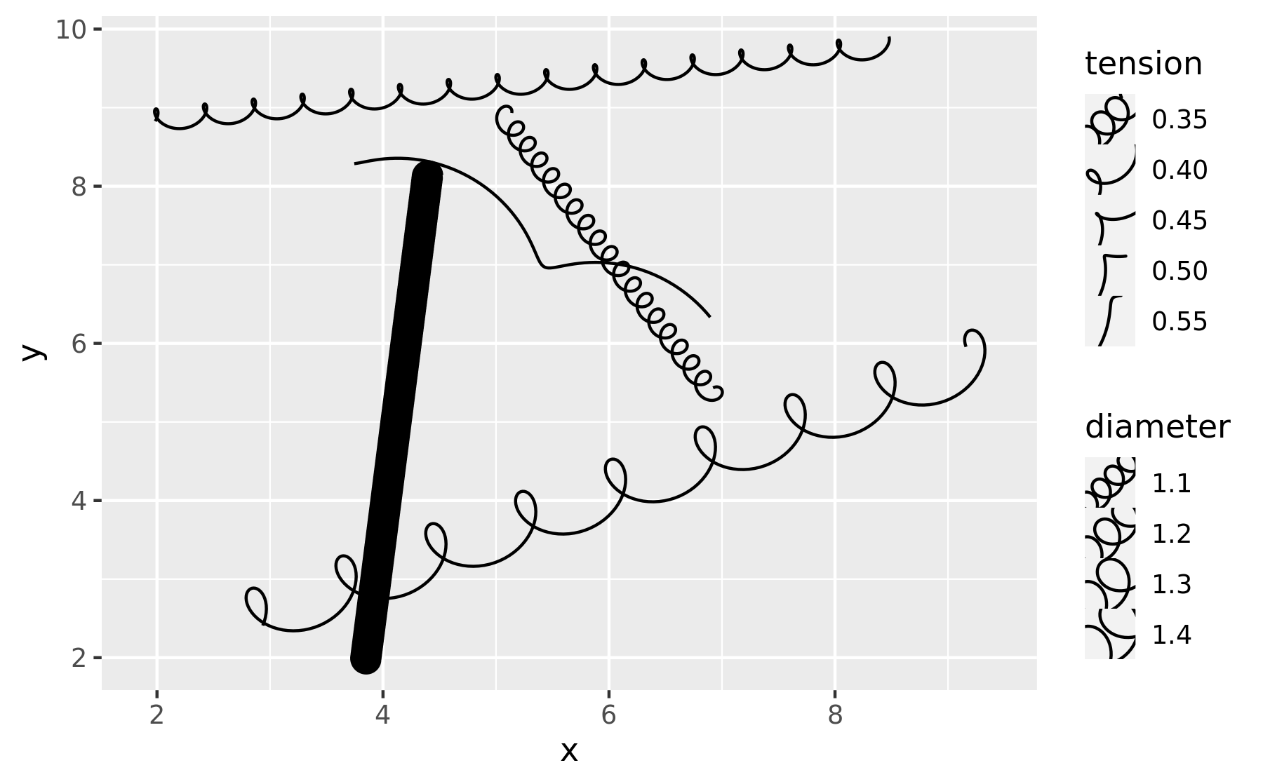
The default key size is a bit cramped for our key, but that has to be modified by the user (ggplot2 doesn’t know about the diameter aesthetic and cannot scale the key size to that in the same way as it does with the size aesthetic).
ggplot(some_data) +
  geom_spring(aes(x = x, y = y, xend = xend, yend = yend, tension = tension,
                  diameter = diameter)) +
  scale_tension(range = c(0.1, 5)) +
  theme(legend.key.size = unit(1, "cm"))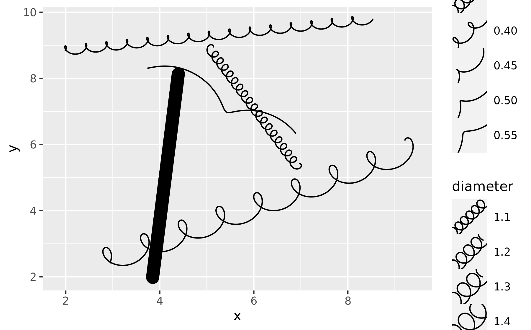
The new legend key will be used for all scaled aesthetics, not just our new diameter and tension meaning that the key will always match the style of the layer:
ggplot(some_data) +
  geom_spring(aes(x = x, y = y, xend = xend, yend = yend, colour = class)) +
  theme(legend.key.size = unit(1, "cm"))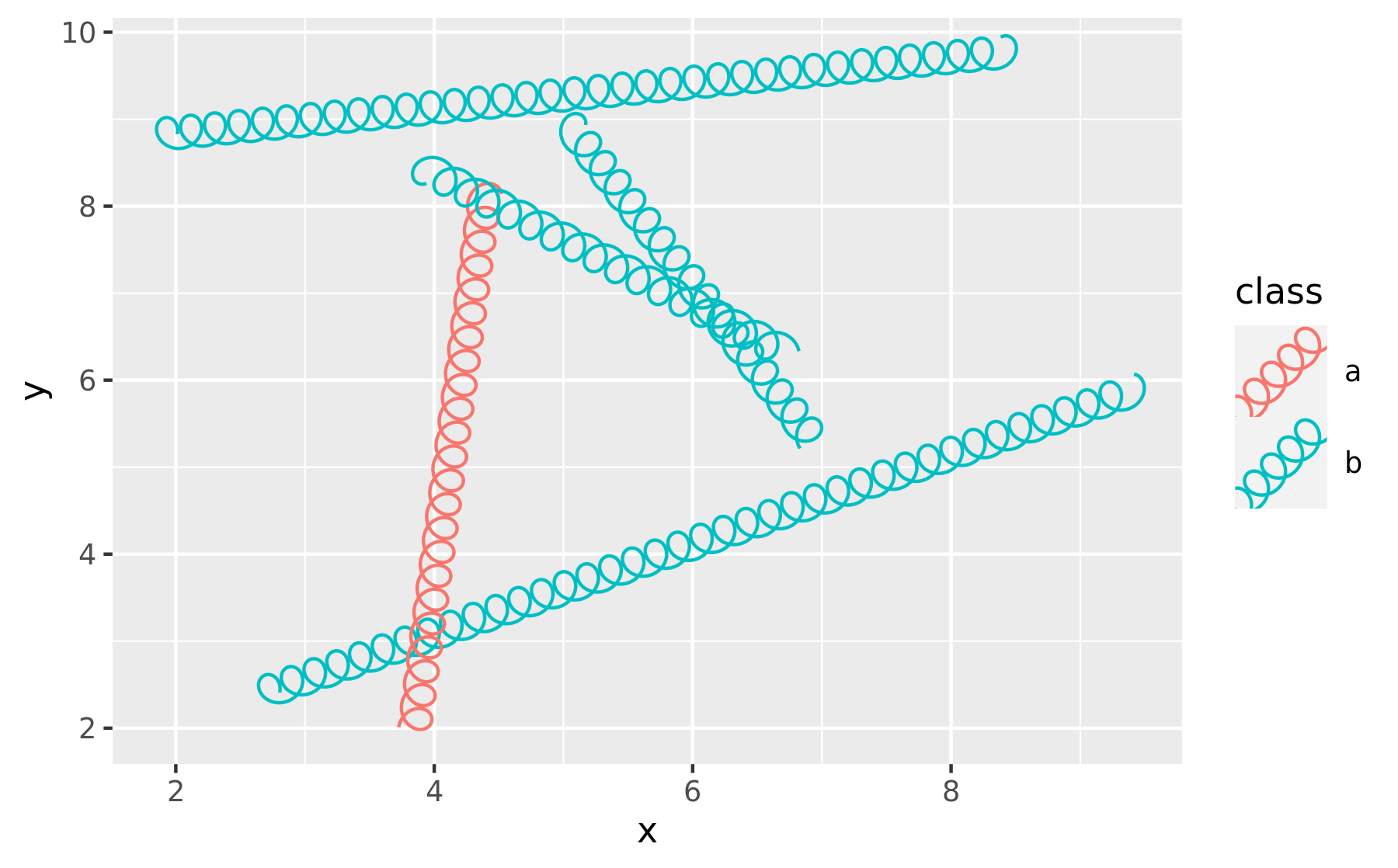
21.6.3 Post-Mortem
This concludes our, admittedly a bit far-fetched, case study on how to create a spring geom. Hopefully it has become clear that there are many different ways to achieve the same geom extension and where you end up is largely guided by your needs and how much energy you want to put into it. While extending layers (and scales) are only a single (but important) part of the ggplot2 extension system, we will not discuss how to create other types of extensions such as coord and facet extensions. The curious reader is invited to study the source code of both ggplot2’s own Facet and Coord classes as well as the extensions available in e.g. the ggforce package.