5.7 Surfaces

So far we’ve considered two classes of geoms:

• Simple geoms where there’s a one-on-one correspondence between rows in the data frame and physical elements of the geom

• Statistical geoms where introduce a layer of statistical summaries in between the raw data and the result

Now we’ll consider cases where a visualisation of a three dimensional surface is required. The ggplot2 package does not support true 3d surfaces, but it does support many common tools for summarising 3d surfaces in 2d: contours, coloured tiles and bubble plots. These all work similarly, differing only in the aesthetic used for the third dimension. Here is an example of a contour plot:

ggplot(faithfuld, aes(eruptions, waiting)) + 
  geom_contour(aes(z = density, colour = ..level..))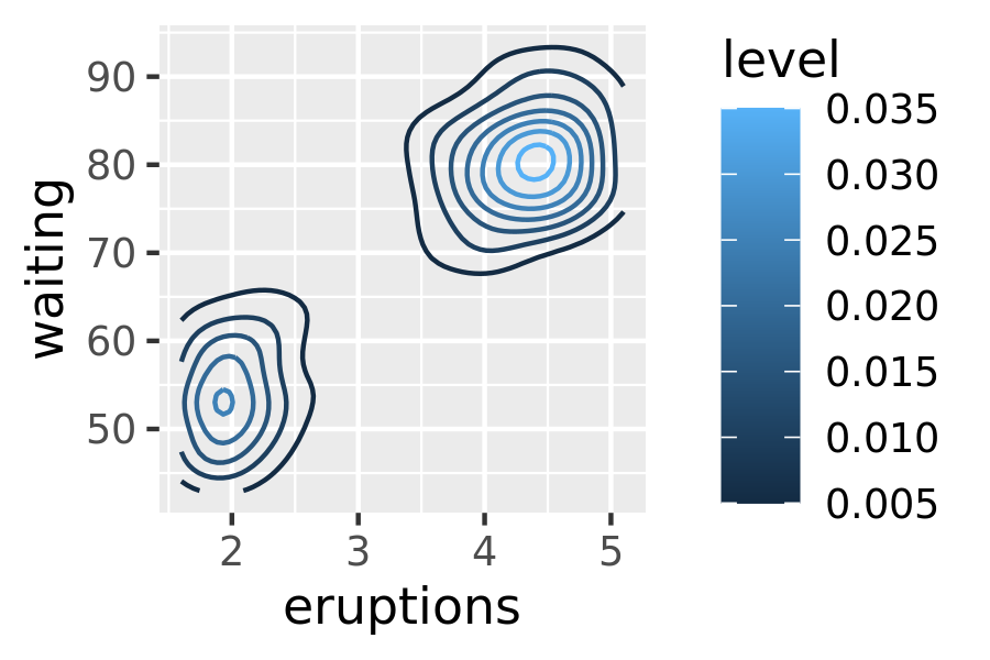

The reference to the ..level.. variable in this code may seem confusing, because there is no variable called ..level.. in the faithfuld data. In this context the .. notation refers to a variable computed internally (see Section 13.6.1). To display the same density as a heat map, you can use geom_raster():

ggplot(faithfuld, aes(eruptions, waiting)) + 
  geom_raster(aes(fill = density))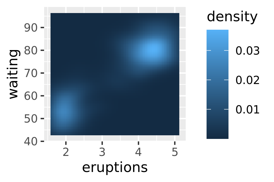

# Bubble plots work better with fewer observations
small <- faithfuld[seq(1, nrow(faithfuld), by = 10), ]
ggplot(small, aes(eruptions, waiting)) + 
  geom_point(aes(size = density), alpha = 1/3) + 
  scale_size_area()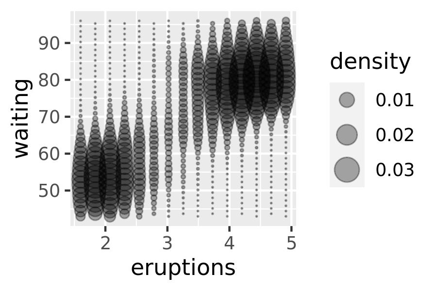

For interactive 3d plots, including true 3d surfaces, see RGL, http://rgl.neoscientists.org/about.shtml.